Introduction

Rendering the teapot was not as such a necessity for this series of basic lessons as it would normally be considered more as an advanced topic. However beside given us an opportunity to learn about the idea that curves and surfaces can be defined in a very compact way using control points weighted by some basis functions (a principle reused by many advanced rendering or shading techniques), it is also very useful to demonstrate that ray tracing is slow as the number of polygons/triangles and objects in the scene increases. The teapot has the advantage of resulting in the creation of 32 polygon grids which we can see as 32 different objects, something that we couldn't have obtained without supporting a parser to read geometry files (which we would rather prefer to ignore for the time being). Because of its increased complexity, this scene now takes a significant amount of time to render. Ray tracers are known for being slow but hopefully a lot of research has also been carried out to address this problem. Most techniques to speed up renders are based on acceleration structures. The most expensive task in a ray tracer is the intersection test. It is a costly operation which is potentially repeated a very large number of times (for each pixel of the frame we need to test all the triangles from the scene). In "Accelerated Ray Tracing" (1983), Fujimoto writes:

Thus, to save time, we need to find ways of reducing this number of intersection tests as much as possible. The principle of acceleration structures, is to help deciding as quickly as possible which objects from the scene a particular ray is likely to intersect and reject large group of objects which we know for certain the ray will never hit. If, with such structure, we can reduce for instance the number of objects that a ray has to test by 50%, then theoretically, we should also roughly cut the render time by two.

Adding Statistics to the Ray Tracer

In order to measure the efficiency of the different acceleration methods we will test in this lesson, we need to be able to compare the render time of a frame with and without acceleration. Gathering some additional statistics like the total number of rays cast in the scene (which is usually directly related to the total render time), the number of times the ray-triangle intersections test has been executed and the number of ray-triangles hits can also give some interesting information: for instance how does the acceleration scheme perform, and which part of the rendering process takes the most time. Making changes to the code to support basic statistics gathering is really straightforward. We won't implement anything fancy here, just a few globals variables to count the number of rays, the number of times the ray-triangle intersection routine is called and the number of ray-triangle hits. Using global variables can be a problem when the application is multi-threaded which is not the case of our code yet. However in the anticipation of this eventuality, we will use atomic operations to modify the content of these variables.

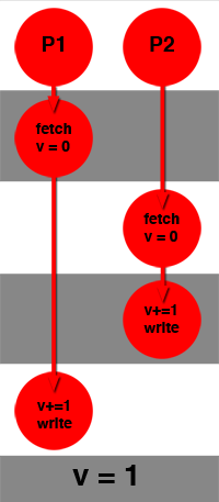
Race conditions may occur when several processors try to update the content of a variable at the same time. Incrementing a variable for example requires to read the variable from memory, increment the value and write the result back to memory. If two processors try to increment a variable v "at the same time", the following sequence of events could happen:

• processor 1 reads variable v from memory (let's assume v = 0) and stalls.
• processor 2 reads variable v from memory = 0, increments the value and writes the result back to memory. The value of v is now 1.
• processor 1 wakes up, increments the value of v which for processor 1 is 0, increment it and write the result to memory. The value of v is still 1, even though it should normally be 2.

It is not possible to stop processor 2 from changing the content of the variable until processor 1 has completed its add operation unless we use a mechanism like a mutex which is overkilled for such simple tasks. For low level tasks such as addition or subtraction, a much better choice to avoid a race condition, is to use atomic operations which have been added to the C++11 standard. Other methods can be used but this is one is really simple to implement. If you are not completely familiar with these concepts, read the lesson on multi-threading.

As for computing the total render time, we can simply keep track of time before the render starts and take the difference with the current time once the frame is finished. In our current implementation, we use the clock() function which does give the CPU time, not the real time. We use the function __sync_fetch_and_add to perform an atomic add (line 10 and 14).

We now have some tools to measure how efficient these acceleration structures are (and compare them to each other, an exercise which is not always very fair. As we will see, the performance of an acceleration method often depends on the scene: a structure which performs well for one particular setup can perform poorly for another. Running our ray tracing with these additions should print out the following statistics at the end of the render:

As expected, the ratio between the number of ray-triangle intersection tests performed and the actual number of hits is really low: 0.002 percent! Let's now see how we can already make things run much faster with some very simple changes.