Random Variables and Probability
Reading time: 13 mins.Statistics and probability are two pretty complex and large topics. Our personal opinion though is that they are very few references or books out there which we believe do explain these fields the right way especially to people who know nothing of the subject. They are either providing tons of pointless examples without explaining the theory, or just give the theory in the form of equations and definitions without really explaining what they mean. We do believe this lesson is one of the best introductions (at least of all the documents we found) on the web so far on probability and statistics.
This lesson is not a complete introduction in statistics. This is more a crash course which hopefully provides enough information on the topic for anybody to understand how, why and where statistical methods and probability are used in rendering (particularly with regard to these Monte Carlo methods).
Random Variables and Probability
The first chapter of this lesson will be dedicated to introducing, explaining and understanding what a random variable is. The concept of random variable is central to the probability theory and also to rendering more specifically. What random variables truly is often misunderstood particularly by programmers who just see them as the result of some C++ functions returning some arbitrary number within a given interval. This is not what a random variable is! Let's take an example and start with a coin. Tossing a coin is an example of what we call a random process, because before you toss that coin, you can't tell or predict whether it will land on heads or tails. This is also true of a rolling die, of roulette, of a lottery game, etc. Even though many natural phenomena can be considered as random processes (the rain falling everyday is a random process), we have mostly mentioned examples of games of chance so far, because they are probably what motivated mathematicians to study and develop statistics and probability theory in the first place. Why? Read this:
The cities of London and Paris were full of shopping opportunities, as well as many chances to lose the family fortune in some high stakes gambling. Games of chance were always popular and the biggest games were found in the larger towns and cities. As a result of all this spending, the nobles always needed more money.
The text here refers to the life and fortune of aristocrats in the 17th and 18th century. In this context, it is not hard to understand why mathematicians of that time got really interested in trying to understand if there was any possible way by which they could measure their chances to win or lose a game of chance, by formalising the process in the form of equations (readers interested in this historical part can search for Comte de Buffon and de Moivre, etc.). Because heads and tails don't fit well in equations, the first thing they did was to map or assign if you wish, numbers to each possible outcome of a random process. In other words, they said lets assign 1 if the coin lands heads up, and 0 if it lands tails up which you can formalize in mathematical notation as:
$$ X(\omega) = \begin{cases} 1, & \text{if} \ \ \omega = \text{heads} ,\\ \\ 0, & \text{if} \ \ \omega = \text{tails} . \end{cases} $$It seems like a very simple idea, but no one had done that before, and this formulation is probably more complex than it appears in the first place. The term \(X\) on the left inside is what you call a random variable. Now notice how we wrote this term as if we had defined it as a function taking the argument \(\omega\). The term \(\omega\) in this context is what we refer to as the outcome of the random process. In our coin example, the outcome can either be "tails" or "heads", in other words, a random variable is a real-valued function mapping a possible outcome (heads or tails) from the random process to a number (1 or 0 but note that these numbers don't need to be 1 and 0 they could be anything else you like such as 12 and 23 or 567 and 1027. What you map the outcome of the process to is really up to you). This is very similar in a way to writing something like \(f(x) = 2x + 3\). A random variable is not a fixed value. It is more like a function, but the word variable in the name makes things confusing because the word variable is generally used to denote unknowns in equations. Maybe it would have been best to call that a random function, but random function in probability theory has another meaning. We are stuck with random variables then however always keep in mind that a random variable is not a fixed value, but a function, mapping or associating a unique numerical value to each possible outcome of a random process which is not necessarily a number ("tails", "heads").
A random variable is a function \(X(e)\) that maps the set of experiment outcomes to the set of numbers.
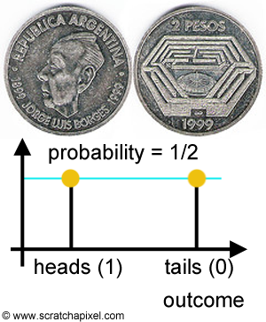
This is not yet the complete definition of a random variable. The other concept associated with the definition of a random variable is the concept of probability. The coin example is convenient because you don't need to be an expert in statistics to know or intuitively agree with the idea that the chances of either getting "heads" or "tails" when you toss a coin are 50-50 (as we commonly say). And that's because no matter how we throw it in the air, it is not going to land on one side more likely than the other. By 50-50, we mean that it is equally likely to land on either "heads" or "tails" (assuming your express chances as a percentage). If you substitute "probability" for "chances" then we can more formally say that the probabilities of getting either heads or tails are \(1\over 2\) and \(1\over 2\) respectively.
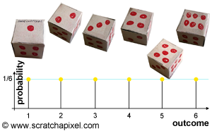
The concept of probability is of course very important because random processes are by definition producing outcomes that are not predictable, however, probabilities can be used to describe the chances for a particular event from a random process to occur. And this is greater than we think, because to something that wasn't predictable and thus usable in mathematics, we now have ways of "quantifying" these events (in the form of probabilities) and manipulating these numbers with mathematical tools to do all sorts of (useful) things. Applied to the case of a rolling die, the probability of getting either 1, 2, 3, 4, 5, or 6 is \(1\over 6\). Generally, the formula to find out the probability of an outcome is 1 divided by the number of possible outcomes (assuming all events are equally likely to happen, which is called equiprobability). In the case of a die, the number of outcomes is 6 (an outcome is any possible result that a random process can produce) thus the probability of either getting 1, 2, ... or 6, any number between 1 and 6, is \(1 \over 6\).
More generally, we can say that if the outcome of some process must be one of \(n\) different outcomes, and if these \(n\) outcomes are equally likely to occur, then the probability of each outcome is \(1 \over n\).
Figures 1 and 2 illustrate the way you can represent the probability associated with each outcome of a random process (such as tossing a coin or rolling a die). On the x-axis, we write down the possible outcomes of the random process and on the y-axis, we write down the probability associated with each one of these outcomes. This is already providing us with a much better definition of a random variable. Not only you can see it as some sort of function mapping outcomes to real values but it also associates a probability value to each one of these outcomes. In others words, \(X\) provides information on the value associated with an outcome of a random process and a value for the probability of that outcome occurring.
Probabilities themselves can be denoted in different ways but often as either \(P\) or \(Pr\). When you see something like this \(Pr(1)\) for instance written in a textbook, this means "what is the probability for the experiment's outcome to be 1?". You could also write \(Pr(odd)\) which you could read as "what is the probability for the outcome of the experiment to be an odd number?" etc. Probabilities themselves can be interpreted in two different ways. You can see them as indicating "how strongly" you believe that some event will be true. However, if you realised that under some given conditions, some outcome occurred 10 times over the 100 times you ran the experiment, then probabilities can also be interpreted as "if you run this experiment 100 times under the same conditions, then you can expect this outcome to occur 10 times". There are quite a few different ways of interpreting probabilties but the "evidential" or Bayesian and "physical" probabilities which we just described are the two most common interpretations.
Terminology
Terminology in statistics is almost everything. There are so many concepts in probability theory and the differences between them are sometimes so subtle, that giving them clear definitions is very important. To paraphrase Wikipedia, in statistics, "confusion results when conventions are not strictly observed". In mathematics, random variables are generally denoted with a capital letter such as \(X, Y, .. Z\). The result of a random process is called an observation or also sometimes realizations or observed value. The process of throwing a die for example is what we call a random process, but the result of that process is what we call an observation, and observations are usually denoted with lowercase letters such as \(x, y, ... z\), etc. If a die is rolled \(n\) times the results of the observations are denoted \(x_1, x_2, ..., x_n\). This definition is slightly different from the definition of an event. A set of possible outcomes from an experiment defines what we call an event. For example, we can say that some event occurred if the result of a die roll is an odd number (that is either 1, 3, or 5). Finally, another important concept related to random variables is the concept of sample space. A sample space defines the set of all possible outcomes from an experiment. For example, in the case of a die, the sample space is defined as \(S = \{1, 2, 3, 4, 5, 6\}\) (the greek letter \(\Omega\) is sometimes also used but we will stick to \(S\) in this lesson). An event can be seen as a subset of the sample space. For instance, if event A is that an odd number is obtained, then A can be defined as \(A = \{1, 3, 5\}\). Finally, each outcome from a set is generally called a member of that set.
Sample space can either be used to define elementary events or non-elementary events. Let's explain. Imagine you have 10 cards labeled and that each card is labeled with the number 0, 1, or 2\. Now let's imagine you have 3 cards labeled 0, 5 cards labeled 1, and 2 cards labeled 2. The sample sample space of non-elementary events is \(S=\{0, 0, 0, 1, 1, 1, 1, 1, 2, 2\}\) and the sample space of elementary events is \(S=\{0, 1, 2\}\).
When you mean that some event has occurred, you potentially mean two things. First that the observation (or outcome from the experiment) satisfies the definition of the event (e.g. if the result of rolling a die is an odd number and the event A is that an odd number is obtained then event A has occurred). And also that the observation which is one of the many possible elements from the sample space, is also an element of that event (if the observation is 3, 3 is an element of subset \(A = \{1, 3, 5\}\)).
Name |
Description |
|---|---|
Random Variable |
A random variable is a function X defined from a sample space S (e.g. "heads", "tails") to a measurable space (1, 0). Random variables are denoted with upper case letters. |
Probability |
A probability provides a quantitative description of the likely occurrence of a particular event. |
Observation or Realization |
A realization, or observed value, of a random variable, is the value that is observed (what happened). Realizations are denoted with lowercase letters (to differentiate them from random variables). |
Event |
An event is any collection of outcomes of an experiment. Any subset of the sample space is an event. |
Sample Space |
An exhaustive list of all the possible outcomes of an experiment. Each possible result of such an experiment is represented by one and only one point in the sample space, which is usually denoted by S. The elements (or members) of the sample space can be thought of as all the different possibilities that could happen. |
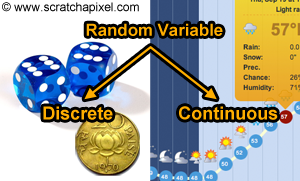
Random variables come in two flavors. They can either be discrete or continuous. When the random variable is discrete, the outcome of the random process can only take a list of exact values. A die roll, a tossed coin, or the number of fishes retained in a net are all examples of experiments whose outcome can only be measured by discrete random variables because they produce a finite or countably infinite several values (the difference between finite and countably infinite is important because although counting how many elements are in a sample space, for instance, may never finish, each element in that sample space might, however, be countable and associated with a number). Temperature measurement can be considered an example of a continuous random variable. Why? Because the possible values that an experiment measuring temperature can take, fall on a continuum. Random variables measuring time and distances are also generally of the continuous type.
Because the topic of statistics and probability is already so large, in this lesson we will mostly focus on discrete random variables. Continuous random variables will be studied in the lesson on importance sampling. In the next chapter, we will introduce what is probably the most important concept associated with random variables (and again in this particular lesson only the case of discrete random variables will be considered): the concept of probability distribution. We will then study the properties of probabilities and some concepts associated with them.