Global Illumination and Path Tracing

Global Illumination and Path Tracing: a Practical Implementation

Global illumination in practice: Monte Carlo path tracing

In the previous chapter, we introduced the principle of Monte Carlo integration to simulate global illumination. We also explained that uniformly sampling the hemisphere works well for simulating indirect diffuse but not for simulating indirect specular or caustics. For this reason, we will limit ourselves to simulating indirect diffuse in this lesson. Diffuse objects illuminate each other as the "indirect" effect of these objects reflecting light themselves and acting somehow as a source of light.

In the first chapter, we showed how the Monte Carlo integration method worked in 2D. Extending the technique to 3D is relatively "simple" and works on the same principle. Here are the steps (which, as you can see, are very similar to the steps we followed in the 2D case).

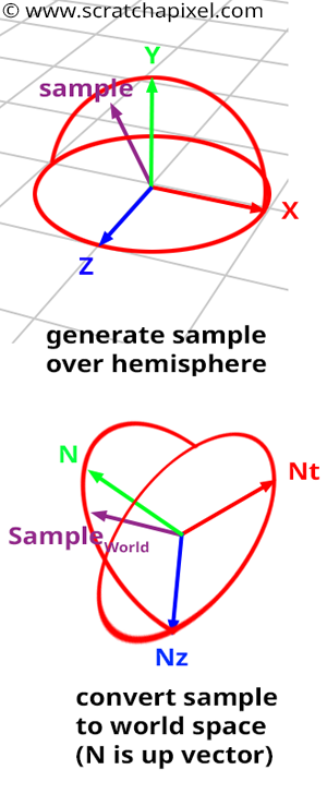
Concept: ideally, we want to create samples on the hemisphere oriented about the normal \(N\) of the shaded point \(P\). Though as in the 2D case, it is easier to create these samples in a hemisphere oriented with the y-axis of some "canonical" Cartesian coordinate systems and then transform them into the shaded point local coordinate system (in which the hemisphere is oriented along the normal as shown in Figure 1 - bottom). The reason why we prefer to create samples in a hemisphere whose up vector is oriented with the y-axis of the world Cartesian coordinate system is that the coordinates of the sample in this coordinate system can be easily computed with the basic spherical-to-Cartesian coordinates equations, which we know are:

And then transformed in the shaded point local coordinate system. We will explain in this lesson how samples are created, how to create a new coordinate system in which the shading normal \(N\) defines the up axis of that coordinate system, and how the other axis of that local Cartesian coordinate system (which are technically tangent to the surface at \(P\) and perpendicular to \(N\)) is also computed. If you read the lesson on Geometry, you should know that once we have the axes of an orthogonal coordinate system \(C\), we can transform any point or vector (aka direction) from any Cartesian coordinate system to \(C\).

• Step 1: Create a Cartesian coordinate system in which the up vector is oriented along the shaded point normal \(N\) (the shaded point normal \(N\) and the up vector of the coordinate system are aligned).

• Step 2: Create a sample using the spherical to Cartesian coordinates equations. We will show in this chapter how this can be done in practice.

• Step 3: transform the sample direction from the original coordinate system to the shaded point coordinate system.

• Step 4: trace a ray in the scene in the sampled direction.

• Step 5: if the ray intersects an object, compute the color of that object at the intersection point and add this result to a temporary variable. Because the surface is diffuse, don't forget to multiply the light intensity returned along each ray by the dot product between the ray direction (the light direction) and the shaded normal \(N\) (see below).

• Step 6: repeat steps 2 to 5 N-times.

• Step 7: divide the temporary variables that hold all the results of all the sampled rays by N, the total number of samples used. The final value approximates the shaded point indirect diffuse illumination: the illumination of \(P\) by other diffuse surfaces in the scene.

In pseudo-code, we get:

Vec3f castRay(Vec3f &orig, Vec3f &dir, const uint32_t &depth, ...)
{
    if (depth > options.maxDepth) return 0;
    Vec3f hitPointColor = 0;
    // compute direct lighting
    ...
    // step1: compute the shaded point coordinate system using normal N.
    ...
    // number of samples N
    uint32_t N = 16;
    Vec3f indirectDiffuse = 0;
    for (uint32_t i = 0; i < N; ++i) {
        // step 2: create a sample in world space
        Vec3f sample = ...;
        // step 3: transform sample from world space to shaded point local coordinate system
        sampleWorld = ...;
        //Steps 4 & 5: cast a ray in this direction
        indirectDiffuse += N.dotProduct(sampleWorld) * castRay(P, sampleWorld, depth + 1, ...);
    }
    // step 7: divide the sum by the total number of samples N
    hitPointColor += (indirectDiffuse / N) * albedo;
    ...
    return hitPointColor;
}

Let's see how to implement these steps one by one.

Step 1: Create a local coordinate system oriented along the shading normal \(N\)

We want to build a Cartesian coordinate system in which the normal \(N\) is aligned with that coordinate system's up vector (or y-axis). What we know from the lesson on Geometry is that a vector can also be interpreted as the coefficients of a plan equation and that the plane in question is perpendicular to that vector:

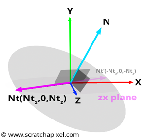
Since we deal with vectors (and not points), the plane passes through the world origin so that we can set D = 0. Since we are looking to build a Cartesian coordinate system, we can assume that any vector on that plane is perpendicular to \(N\). Let's call this vector \(N_T\). We could use \(N_T\) as the second axis of our coordinate system. Now by taking the cross product of \(N_T\) and \(N\) we would create a third vector \(N_B\) perpendicular to both \(N_T\) and \(N\). Et voila! \(N\), \(N_T\) and \(N_B\) form a Cartesian coordinate system. So how do we find a vector lying in the plane anyway?

In Figure 3, you will realize that one of the vectors lying in the plane has its y-coordinate equal to 0. So we can assume that there is one such vector lying in this plane whose y-coordinate is 0, which reduces our plane equation to two unknowns:

We can re-write this equation as follows:

Note that this equation is true if \(x = N_z\) and \(z = -N_x\) or if \(x = -N_z\) and \(z = -N_x\). So this is simple, if we take either \(N_T = {N_z, 0, -N_x}\) or \(N_T = {-N_z, 0, N_x}\), then we have a vector lying in the plane perpendicular to \(N\). You can choose either option as long as you create a right-hand coordinate system which also depends on the order in which you order \(N\) and \(N_T\) in the final cross product. The only thing we need to take care of is to normalize \(N_T\):

void createCoordinateSystem(const Vec3f &N, Vec3f &Nt, Vec3f &Nb)
{
    Nt = Vec3f(N.z, 0, -N.x) / sqrtf(N.x * N.x + N.z * N.z);
    ...
}

All there is left now is to compute \(N_B\) with a cross product:

void createCoordinateSystem(const Vec3f &N, Vec3f &Nt, Vec3f &Nb)
{
    Nt = Vec3f(N.z, 0, -N.x) / sqrtf(N.x * N.x + N.z * N.z);
    Nb = N.crossProduct(Nt); 
}

However, this construction is not the best if the normal vector's y-coordinate is greater than its x-coordinate. In this particular case, it is best for numerical robustness to build a vector within the plane whose x-coordinate is equal to 0. If you watch Figure 3 again, you will see that this is also an option:

The same logic applies here to find a possible solution for y and z. Finally, we get:

void createCoordinateSystem(const Vec3f &N, Vec3f &Nt, Vec3f &Nb) 
{ 
    if (std::fabs(N.x) > std::fabs(N.y))
        Nt = Vec3f(N.z, 0, -N.x) / sqrtf(N.x * N.x + N.z * N.z);
    else
        Nt = Vec3f(0, -N.z, N.y) / sqrtf(N.y * N.y + N.z * N.z);
    Nb = N.crossProduct(Nt); 
}

Our local coordinate system is built! Now, we have to learn how to create samples and then transform these samples in this coordinate system.

Create samples on the hemisphere

As you know, we can define the position of a point on the sphere (or hemisphere) using either polar coordinates or Cartesian coordinates. In polar coordinates, a point or a vector (we are interested in direction here) is defined with two angles: \(\theta\) (the Greek letter theta) and \(\phi\) (the Greek letter phi). The first angle is contained in the range \([0,\pi/2]\) and the second angle (\(\phi\)) is contained in the range \([0,2\pi]\). Remember that the Monte Carlo integration method works if we randomly choose the samples' direction. Now, this is where the Monte Carlo theory kicks in. Remember that what we want to do here is uniformly sample the hemisphere with respect to the solid angle. Now we won't explain the theory of Monte Carlo again in this section. If you haven't read the lesson on Monte Carlo yet, now is the time to do so (Mathematical Foundations of Monte Carlo Methods and Monte Carlo in Practice). Anyway, be ready: we will have to deal with some maths now.

Now the actual equation (which is called an estimator) that we are going to be using looks as follows (read "the Monte Carlo estimator for the integral of the function f(x), with probability density function pdf(x) is"):

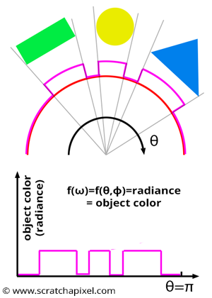
This is the generic form of a Monte Carlo estimator that we can use to approximate an integral result. What we want to integrate into this particular case is the function \(f(x)\). As explained in the previous chapter, in our case, this function can be seen as the amount of light arriving at \(P\), the shaded point from every direction in the hemisphere oriented around the normal at \(P\). It is simpler to imagine what this function can look like if you consider the 2D case (or a slice through the hemisphere), as shown in Figure 4. Now, the idea here is to sample that function for random directions. In the equation above, this is represented by the random variable \(X_i\). So the idea is that we generate a random direction \(D_R\) in the hemisphere and evaluate the function for that direction, which in our case means "cast the ray from \(P\) in the direction \(D_R\) into the scene and return the color of the object that this ray intersected (if it intersected an object at all)". That color represents the amount of light that the object the ray intersected reflects towards \(P\) along the ray direction \(D_R\). Mathematically we also need to divide this result by the probability of generating the direction \(D_R\). This is represented in the equation above by the term called PDF (this stands for probability distribution function). The result of this function could be unique for each random direction \(X_i\). This is why it is defined as a function. Hopefully, because we want to generate uniformly distributed samples (or directions), all the rays will have the same PDF. In this case, the PDF is constant because all rays or directions have the same probability of being generated (we speak of equiprobability). So let's find this PDF and learn how to generate these random, uniformly distributed samples or directions.

To sample a function, we need first to find the PDF of that function, then compute its CDF then finally, the inverse of that CDF. These steps were explained in detail in the lesson Mathematical Foundations of Monte Carlo Methods; keep in mind that we want to sample the hemisphere uniformly. That means that any of the samples or directions we draw should have the same probability as any other. The probability of drawing direction A is the same as that of drawing direction B, C, D, etc. The probability of drawing a sample from a given function is given by the function's PDF (probability distribution function). We also know that all PDFs must integrate to 1 over their sample space (or domain of integration). In the case of the hemisphere, we will first define that sample space in terms of solid angle: the solid angle of a hemisphere is equal to \(2\pi\). And since all samples have the same chance (aka probability) of being generated, then our PDF must also be constant. If we write our PDF as \(p(x)\) and then integrate it over the entire sample space (\(2 \pi\)), then we get (where again we will express values in terms of solid angle to start with):

Because as mentioned before, a PDF must integrate to 1 over the function sample space. Since \(p(\omega)\) is a constant, we can write (we replace the PDF by the constant C in the following equation):

We know (check the lesson the Mathematic of Shading in the section Mathematics of Computer Graphics) that:

Thus:

From which we can find C or the PDF of our function:

So far, so good. Now it's great to know the PDF of the function we want to sample to start with, but the problem is that we can't work with solid angles. Our ultimate goal is to generate random directions contained within the hemisphere, so we need to express this PDF in terms of polar coordinates, i.e., in terms of \(\theta\) and \(\phi\):

Now we know that the probability that a given solid angle belongs to a larger set can be written as:

This is just a generalization of the equation we integrated above, but in the previous equation, \(\omega\) was equal to \(2\pi+\); in other words, \(\omega\) covered the area of the entire hemisphere. Now, if we want to express the same probability density function but this time in terms of \(\theta\) and \(\phi\), we can write:

We learned in the previous lesson that a differential solid angle can be re-written in terms of polar coordinates as follows:

If we substitute this equation in the previous equation, we get:

The \(d \theta\) and \(d \phi\) on each side of the equation cancel out, and we get:

We just replaced \(p(\theta)\) with the value we computed above: \(p(\omega) = 1 / 2\pi\). With a little more patience, we are almost there. The function \(p(\theta, \phi)\) is called a joint probability distribution. Now, we need to sample \(\theta\) and \(\phi\) independently. In this particular case, the PDF is said to be separable. In other words, we can split the PDF into two PDFs, one for \(\theta\) and one for \(\phi\), but we can also use another technique, which relies on the concept of marginal and conditional PDF. A marginal distribution is one in which the probability of a given variable (for example \(\theta\)) can be expressed without any reference to the other variables (for example \(\phi\)). You can do this by integrating the given PDF with respect to one of the variables. In our case, we get (will integrate \(p(\theta, \phi\)) with respect to \(\phi\)):

The conditional probability function gives the probability function of one of the variables (for example, \(\phi\)) when the other variable (\(\theta\)) is known. For continuous functions (which is the case of our PDFs in this example), this can be computed as the joint probability distribution \(p(\theta, \phi)\) over the marginal distribution \(p(\theta)\):

Now that we have the PDFs for \(\theta\) and \(\phi\), we need to find their respective CDFs (and the inverse of these CDFs). Remember from the lesson on Monte Carlo that a CDF can be seen as a function that returns the probability that some random variable \(X\) will be found to have a value less or equal to \(x\). To take a practical example, let's say "if I randomly generate a random value for \(\theta\), what is the probability that \(\theta\) takes on a value less than or equal to, say, for example, \(\pi/4\)? We can compute this CDF as an integral of the PDF as follows:

The Fundamental Theorem of Calculus says that if \(f (x)\) is continuous on [a, b] and if If \(F(x)\) is any antiderivative of \(f(x)\), then $$\int_{a}^{b} f(x) \, dx = F(b) - F(a).$$

The antiderivative of \(\sin x\) is \(-\cos x\), thus:

The CDF of the \(p(\phi)\) is simpler:

Let's finally invert these CDFs:

Congratulation. The rest of the Monte Carlo theory now tells us that if we draw some random variable uniformly distributed in the range [0,1], and replace these random numbers in the equations above, then we get uniformly distributed values of \(\theta\) and \(\phi\) which we can then use in the polar-to-Cartesian coordinates equations to compute a random uniformly distributed direction over the hemisphere. Let's see how this works in practice:

Vec3f uniformSampleHemisphere(const float &r1, const float &r2)
{
    // cos(theta) = r1 = y
    // cos^2(theta) + sin^2(theta) = 1 -> sin(theta) = srtf(1 - cos^2(theta))
    float sinTheta = sqrtf(1 - r1 * r1);
    float phi = 2 * M_PI * r2;
    float x = sinTheta * cosf(phi);
    float z = sinTheta * sinf(phi);
    return Vec3f(x, r1, z);
}

...
std::default_random_engine generator;
std::uniform_real_distribution<float> distribution(0, 1);

uint32_t N = 16;

for (uint32_t n = 0; n < N; ++i) {
    float r1 = distribution(generator);
    float r2 = distribution(generator);
    Vec3f sample = uniformSampleHemisphere(r1, r2);
    ...
}

There is a couple of interesting things to note about the code above. Note that when we inverted the first CDF one of the equations was \(\cos \theta = 1 - y\). The \(y\) variable is the random variable uniformly distributed between 0 and 1 that we want to use to randomly pick a value for \(\theta\). So \(1 - y\) or \(1 - \epsilon\) if \(\epsilon\), the Greek letter epsilon which represents our uniformly distributed random variable, is equal to \(\cos \theta\). First, \(\cos \theta\) is the y-coordinate of the random direction. So we can directly set the y-coordinate of our random direction with \(1 - \epsilon\) (line 9). Then note that \(\cos^2 \theta + \sin^2 \theta = 1\) thus \(\sin \theta = \sqrt{1 - cos^2 \theta}\). If we replace \(\cos \theta\) with \(1 - \epsilon\) again, then we get \(\sin \theta = \sqrt{1 - (1-\epsilon) * (1-\epsilon)}\). Then finally, note that because our random variable \(\epsilon\) is uniformly distributed using \(1-\epsilon\) or \(\epsilon\) is the same. It doesn't matter since there is as much probability to draw a \(1 - \epsilon\) than a \(\epsilon\). Since both numbers have the same probability of being generated, one can be used in place of the other (and vice versa). This simplifies our equation to \(\cos \theta = \epsilon\) and \(\sin \theta = \sqrt{1 - \epsilon * \epsilon}\).

Great, it was a lot of maths, but now you know how to generate uniformly distributed random samples in the hemisphere. Let's move to the next step and transform this sample to the shaded point local coordinate system.

Step 3: transform the random samples to the shaded point local coordinate system.

We already computed a local coordinate Cartesian system in which the normal of the shaded point is aligned with the up vector of that coordinate system. As we know from the lesson on geometry, the three vectors of that Cartesian coordinate system can be used to build a 4x4 matrix (or 3x3 matrix if we only care about directions) that will transform a direction from whatever space that direction is initially in, to the coordinate system from which we built the transformation matrix.

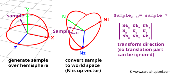
In this particular case, we will use the vectors of the Cartesian coordinate system directly without building a matrix (if you are unsure about how this part of the code works, we recommend that you read the lesson on Geometry):

Vec3f Nt, Nb;

createCoordinateSystem(hitNormal, Nt, Nb);

for (uint32_t n = 0; n < N; ++i) {
    float r1 = distribution(generator); // cos(theta) = N.Light Direction
    float r2 = distribution(generator);
    Vec3f sample = uniformSampleHemisphere(r1, r2);
    Vec3f sampleWorld( 
        sample.x * Nb.x + sample.y * hitNormal.x + sample.z * Nt.x,
        sample.x * Nb.y + sample.y * hitNormal.y + sample.z * Nt.y,
        sample.x * Nb.z + sample.y * hitNormal.z + sample.z * Nt.z);
    ...
}

Steps 4, 5, and 6: trace the indirect rays.

The next step is to trace the ray and accumulate the returned color into a temporary variable. Once all the rays have been traced, we divide this temporary variable in which the result of all the rays accumulated (the amount of light returned along each indirect cast ray) by N, the total number of samples.

Vec3f indirectDiffuse = 0;
for (uint32_t n = 0; n < N; ++i) {
    float r1 = distribution(generator); // cos(theta) = N.Light Direction
    float r2 = distribution(generator);
    Vec3f sample = uniformSampleHemisphere(r1, r2);
    ...
    // don't forget to apply cosine law (i.e., multiply by cos(theta) = r1).
    // we should also divide the result by the PDF (1/2*M_PI), but we can do this after
    indirectDiffuse += r1 * castRay(hitPoint + sampleWorld * options.bias, 
        sampleWorld, depth + 1, ...);
}
// divide by N and the constant PDF
indirectDiffuse /= N * (1 / (2 * M_PI));

Don't forget that the light intensity returned along the direction sampleWorld also needs to be multiplied by the cosine of the angle between the shaded normal and the light direction (which is the ray direction in this case). Because our object is diffuse, we need to apply the cosine law (which we introduced in the first lesson on shading). Remember that the random variable r1 is equal to \(\cos \theta\), which is the cosine of the angle between \(N\) and the ray direction (check the code of the function uniformSampleHemisphere). So all there is to do in this case is multiply the result of castRay (the amount of light reaching \(P\) from the direction sampleWorld) by r1 (line 8).

Step 7: add the contribution of the indirect diffuse to the illumination of the shaded point

Final touch. Add the result of the indirect diffuse calculation to the total illumination of the shaded point and multiply the sum of the direct and indirect illumination by the object albedo.

hitColor = (directDiffuse + indirectDiffuse) * object->albedo / M_PI;

Don't forget that the BRDF of a diffuse surface is \(\rho/\pi\) where \(\rho\) stands for the surface albedo. So we need to divide the result by \(\pi\). Though in the case of the indirect diffuse component, don't forget that we should have divided the result of castRay by the PDF of the random variable, which, as we showed earlier in this chapter, is \(1/(2\pi)\). Dividing indirectDiffuseby \(1/(2\pi)\) is the same as multiplying this value by \(2\pi\). And since the albedo is also divided by \(\pi\), we can simplify the code above with:

// (indirectDiffuse / (1 / 2 * M_PI) + directDiffuse) * albedo / M_PI
// (2 * M_PI * indirectDiffuse + directDiffuse) * albedo / M_PI
// (2 * indirectDiffuse + directDiffuse / M_PI) * albedo
hitColor = (directDiffuse / M_PI + 2 * indirectDiffuse) * object->albedo;

ET VOILA!

Monte Carlo path tracing: results.

Let's now see some results. You can find the source code used to render the scene below in the last chapter of this lesson (as usual). In the image below, you can see two renders: on the left, global illumination was turned off, and on the right, it was turned on. Arrows in the image indicate part of the image in which the effect of other surfaces illuminating other objects in the scene can be seen, such as the effect of the floor on the bottom right part of the sphere or the effect of the green monolith on the left side of the sphere. Notice how the sphere takes on the floor's and monolith's red or green color: the term color bleeding is often used to describe this phenomenon (because the color of objects bleeds onto others).

The render time is already significantly slower compared to the time it takes to render direct lighting alone. Thus, in this example, we have limited the number of bounces to 1; you can experiment with a higher number of bounces (if you are patient enough to wait for the result).

Monte Carlo path tracing is slow and noisy.

As you can see in the images below, Monte Carlo path tracing produces noisy images. This is the main problem with this technique. Why? If we go back to our poll example, if you choose a sample of 1,000 different persons to estimate the average weight of a given population, each time you run the poll, you are likely to get 1,0000 other people. And thus, each time you compute the average of a new sample, you will get a "slightly" different number (two samples of 1,000 individuals may as well have the same average weight but call this luck). So if you compute the average of 10 groups of 1,000 adults, you will get 10 different approximations. This is where the noise comes from. There is always more or less variation between what the exact result should be (which is what we want to compute with the integral) and the result of the Monte Carlo integral, which is just an approximation. This variation is what produces noise in the image.

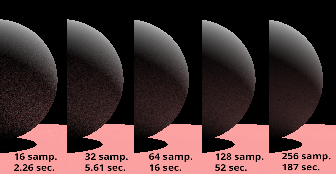
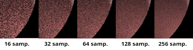
How significant the variation depends essentially on the sample size, the number N. By increasing N, we can reduce the noise in the image. The image above shows a close-up of the sphere for different values of N. As N increases, you can see that the noise becomes less visible. However, this has a cost since rendering time increases with the number of samples used. Monte Carlo theory tells us that to reduce some noise level (called variance) by 2, you need 4 times more samples than the number of samples used in the first place. In other words, to reduce the noise of the first image on the left by 2, you don't need 32 samples but 64 samples, and to halve the noise in the image rendered with 128 samples, you would need 512 samples. You can find why in the lesson Mathematical Foundation of Monte Carlo methods.

How Do I know that my implementation does the right thing? The furnace test.

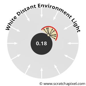
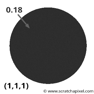
When you implement the technique we described in this lesson, you want to be sure that your implementation is correct. One simple method for testing your implementation is to render a 0.18 grey ball (or 0.5, for that matter. It doesn't make much difference) inside a "white spherical environment". Imagine, for instance, that your grey sphere is surrounded by a larger white sphere emitting light. In our program, we can simulate this easily by making the castRay() return 1 when rays don't intersect geometry and render the image of the grey sphere. What would you expect the result to be? Well, theory tells us that if the object is diffuse, then the albedo of an object can be seen as the amount of light it reflects over the amount of light it receives. In this setup, each point on the grey sphere receives "white" light from all the directions in the hemisphere oriented about the normal at that point. This light or energy is also reflected in all directions in this hemisphere. This is how diffuse surfaces reflect light. Thus, logically if a point receives "white" from all directions and reflects 18% of that incoming light in all directions (if the sphere's albedo is 0.18), then we would expect each point on the sphere to have an intensity of 0.18 exactly.

This is a simple test you can do. Render a 0.18 grey sphere in a white environment. The render of the sphere should look like the render in Figure 6. The sphere should have constant intensity across its surface, and you should read an intensity of 0.18. If this is not the case, your code is not working correctly. Of course, if you use Monte Carlo integration to render this image, each pixel in the sphere may have a slightly different intensity, but as N increases, it should converge to 0.18.

Many things can go wrong when you implement global illumination. Still, the most common mistakes are: you forget to divide the illumination function by the PDF of the random variable, the random variables are not generated with the proper distribution, you forget to multiply the light intensity (light energy traveling along the light direction which as we mentioned before is called radiance) by the cosine of the angle between the light direction and the surface normal, etc.

Vec3f castRay(
    const Vec3f &orig, const Vec3f &dir,
    ...)
{
    if (trace(orig, dir, objects, isect)) {
        ...
        switch (isect.hitObject->type) {
            case kDiffuse:
            {
                ...
                Vec3f indirectLigthing = 0;
#ifdef GI
                uint32_t N = 128;// / (depth + 1);
                Vec3f Nt, Nb;
                createCoordinateSystem(hitNormal, Nt, Nb);
                float pdf = 1 / (2 * M_PI);
                for (uint32_t n = 0; n < N; ++n) {
                    float r1 = distribution(generator);
                    float r2 = distribution(generator);
                    Vec3f sample = uniformSampleHemisphere(r1, r2);
                    Vec3f sampleWorld( 
                        sample.x * Nb.x + sample.y * hitNormal.x + sample.z * Nt.x,
                        sample.x * Nb.y + sample.y * hitNormal.y + sample.z * Nt.y,
                        sample.x * Nb.z + sample.y * hitNormal.z + sample.z * Nt.z);
                    // don't forget to divide by PDF and multiply by cos(theta)
                    indirectLigthing += r1 * castRay(hitPoint + sampleWorld * options.bias,
                        sampleWorld, objects, lights, options, depth + 1) / pdf;
                }
                // divide by N
                indirectLigthing /= (float)N;
#endif

                hitColor = (directLighting + indirectLigthing) * isect.hitObject->albedo / M_PI;
                break;
            }
            ...
        }
    }
    else {
        // return white (as if a white spherical light illuminated the grey sphere)
        hitColor = 1;
    }

    return hitColor;
}

int main(int argc, char **argv)
{
    ...
    
    Sphere *sph = new Sphere(Matrix44f::kIndentiy, 1);
    sph->albedo = 0.18;
    objects.push_back(std::unique_ptr<Object>(sph));
    
    // finally, render
    render(options, objects, lights);

    return 0;
}

Unbiased path tracing: what does it mean?

You may have heard the term "biased" or "unbiased" path tracing, but what does it mean? These concepts have already been introduced in the lesson Mathematical Foundations of Monte Carlo Methods. You can use different estimators than the one we used in this lesson. The one we used here was:

It is a good estimator because it converges in probability to the exact solution (the real solution of the integral), but it converges slowly. As explained above, you need four times more samples each time you want to halve the noise in the image. Other estimators exist. They have the advantage of converging faster but at the price of introducing a "small" bias in the result. In other words, they will provide a result close to the actual result but slightly above or below the exact number. These estimators are said to be "biased". When you write a renderer, if being "physically accurate" is not an absolute requirement, it might be better to use a "biased" estimator, as it makes it possible to get an image that is potentially less noisy (or not noisy at all in some cases) at a fraction of the time it would take to render an image of the same quality using an "unbiased" estimator. When you write a production renderer, you often have to find a tradeoff between "accuracy" and speed.

Environment and image-based lighting.

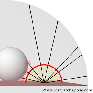
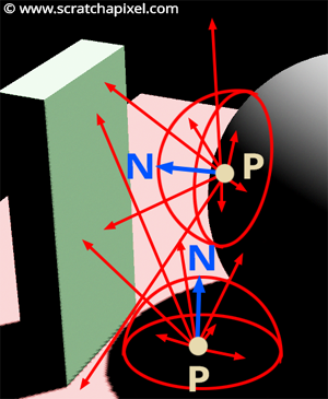
It is possible to make a simple change to the code to implement a feature called environment lighting. The idea is to simulate somehow the illumination of objects by their environment, which in the real world can be something like the sky and all the other objects surrounding a given object you are looking at. The idea is to surround the CG objects with a spherical light source. This spherical light source can emit light uniformly all across its surface. To evaluate the contribution of this light source, we will use the Monte Carlo integration technique again. For each shaded point (or intersection point hit by a primary ray), we will cast N rays uniformly distributed in the hemisphere oriented about the shading normal. In some cases, these rays will hit an object. In this case, the object this ray intersected is blocking light emitted by the spherical light source from reaching the shading point, as shown in Figure 8. When the ray doesn't intersect any geometry, we can assume that the spherical light and the shading point are visible to each other and that \(P\) is illuminated by that light for the direction defined by the ray (Figure 8).

We assume, in this example, that the spherical light source is infinitely far away from the shading points. And thus, the square falloff rule doesn't apply. Such lights are called distant environment light and are typically used in CG to simulate the lighting of objects in their distant environment.

We can use this technique to compute how much light from the spherical light reaches \(P\). This gives us the image below on the left:

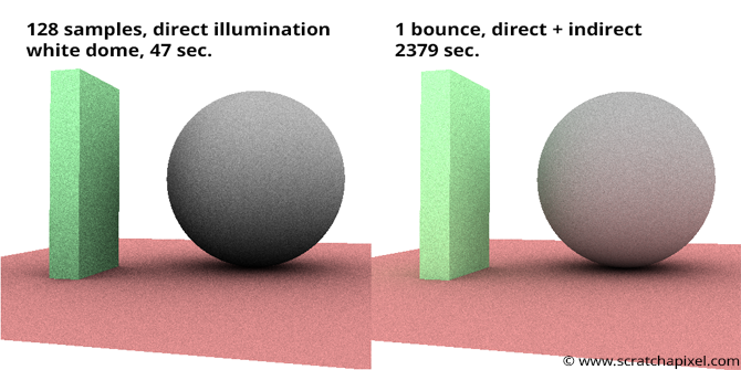
While we have been using Monte Carlo integration in this particular to compute direct illumination (the illumination of each point in the scene by the spherical light source), we can also activate global illumination and calculate the amount of light reflected by objects in the scenes, each time a ray cast from \(P\) to compute direct illumination intersects an object. This can become very expensive as the number of bounces increases. Adding direct and indirect illumination using a white environment light can be seen in the image above on the right.

Why is it called Monte Carlo path tracing?

After all these explanations, this should be obvious to you now. Monte Carlo because we use Monte Carlo methods to solve global illumination, which can be defined mathematically as an integral. This integral means "collect all light illuminating \(P\) for all the directions contained in the hemisphere above \(P\)". Path tracing is simply because we simulate light paths, the natural path of light rays as they bounce from surface to surface (or interact with various materials: glass, water, specular surfaces, etc.). The technique we described in this lesson is one kind of light transport. It is also called unidirectional path tracing because we only follow the path of light rays in one single direction: from the eye back to the light sources. As you may have guessed, there is another algorithm called bidirectional path-tracing, which consists of tracing some light rays from the eyes to the objects in the scene, other rays from the light sources to the objects in the scene, and connecting the two types of rays to form complete light paths. This method can better simulate indirect specular reflections or caustics and will be described in the next section.

Congratulation! Knowing so much about rendering already is quite an achievement. You have learned about light transport, Monte Carlo integration, BRDF, and path tracing in just a few lessons. These are some of the most challenging concepts to understand in computer graphics.

Conclusion.

• The principle of Monte Carlo integration to simulate global illumination is simple.

• Though getting the maths right can be tricky. It generally requires knowing Monte Carlo theory well and what a PDF, a CDF, an estimator, and the inversion sampling method are. Though luckily for you, all these things are explained in great detail in our two lessons devoted to Monte Carlo methods (theory and practice).

• Ray-Tracing is expensive. Monte Carlo path tracing uses many rays and is thus costly, too, especially as the number of samples used or bounces increases. This show the importance of accelerating ray tracing. We will speak about this in the next section.

• Noise is the main problem of Monte Carlo path-tracing. In the next section, we will also show techniques to reduce noise.

• Monte Carlo integration can also simulate direct lighting from distant environment lights (image-based lighting is based on that idea).

You can find more information on all these topics in the next section.

Reference:

The Rendering Equation. Siggraph 1986, James T. Kajiya.