Ray-Sphere Intersection
Reading time: 18 mins.Intersecting a ray with a sphere is the simplest form of a ray-geometry intersection test, which is why many ray tracers showcase images of spheres. Its simplicity also lends to its speed. However, to ensure it works reliably, there are always a few important subtleties to pay attention to.
This test can be implemented using two methods. The first solves the problem using geometry. The second technique, often the preferred solution (because it can be reused for a wider variety of surfaces called quadric surfaces), utilizes an analytic (or algebraic, e.g., can be resolved using a closed-form expression) solution.
Geometric Solution
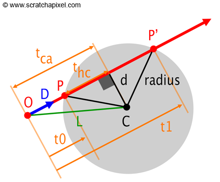
The geometric solution to the ray-sphere intersection test relies on simple math, mainly geometry, trigonometry, and the Pythagorean theorem. If you look at Figure 1, you will understand that to find the positions of the points P and P', which correspond to the points where the ray intersects the sphere, we need to find values for \(t_0\) and \(t_1\).
Remember that a ray can be expressed using the following parametric form:
$$O + tD$$Where \(O\) represents the origin of the ray, and \(D\) is the ray direction (usually normalized). Changing the value of \(t\) allows defining any position along the ray. When \(t\) is greater than 0, the point is located in front of the ray's origin (looking down the ray's direction); when \(t\) is equal to 0, the point coincides with the ray's origin (O), and when \(t\) is negative, the point is located behind its origin. By looking at Figure 1, you can see that \(t_0\) can be found by subtracting \(t_{hc}\) from \(t_{ca}\), and \(t_1\) can be found by adding \(t_{hc}\) to \(t_{ca}\). All we need to do is find ways of computing these two values (\(t_{hc}\) and \(t_{ca}\)) from which we can derive \(t_0\), \(t_1\), and then P and P' using the ray parametric equation:
$$ \begin{array}{lcl} P & = & O + t_{0}D\\ P' & = & O + t_{1}D \end{array} $$We will start by noting that the triangle formed by the edges \(L\), \(t_{ca}\), and \(d\) is a right triangle. So, we can easily calculate \(L\), which is just the vector between \(O\) (the ray's origin) and \(C\) (the sphere's center). \(t_{ca}\) is yet to be determined, but we can use trigonometry to solve this problem.
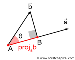
We know \(L\), and we know \(D\), the ray's direction. We also know that the dot (or scalar) product of a vector \(\vec{b}\) and \(\vec{a}\) corresponds to projecting \(\vec{b}\) onto the line defined by vector \(\vec{a}\), and the result of this projection is the length of the segment AB as shown in Figure 2 (for more information on the properties of the dot product, check the Geometry lesson):
$$\vec{a} \cdot \vec{b} = |a||b|\cos\theta.$$In other words, the dot product of \(L\) and \(D\) gives us \(t_{ca}\). Note that there can only be an intersection between the ray and the sphere if \(t_{ca}\) is positive (if it is negative, it means that the vector \(L\) and the vector \(D\) point in opposite directions. If there is an intersection, it could be behind the ray's origin, but anything happening behind it is of no use to us). We now have \(t_{ca}\) and \(L\).
$$ \begin{array}{l} L = C - O\\ t_{ca} = L \cdot D\\ if \; (t_{ca} < 0) \; return \; false \end{array} $$There is a second right triangle in this construction, defined by \(d\), \(t_{hc}\), and the sphere's radius. We already know the radius of the sphere, and we are looking for \(t_{hc}\) to find \(t_0\) and \(t_1\). To get there, we first need to calculate \(d\). Remember, \(d\) is also the opposite side of the right triangle defined by \(d\), \(t_{ca}\), and \(L\). The Pythagorean theorem states that:
$$\text{opposite side}^2 + \text{adjacent side}^2 = \text{hypotenuse}^2$$Replacing the opposite side, adjacent side, and hypotenuse respectively with \(d\), \(t_{ca}\), and \(L\), we get:
$$ \begin{array}{l} d^2 + t_{ca}^2 = L^2\\ d = \sqrt{L^2 - t_{ca}^2} = \sqrt{L \cdot L - t_{ca} \cdot t_{ca}}\\ if \; (d < 0) \; return \; false \end{array} $$Note that if \(d\) is greater than the sphere's radius, the ray misses the sphere, indicating no intersection (the ray overshoots the sphere). Now we have all the terms needed to calculate \(t_{hc}\). Using the Pythagorean theorem again:
$$ \begin{array}{l} d^2 + t_{hc}^2 = \text{radius}^2\\ t_{hc} = \sqrt{\text{radius}^2 - d^2}\\ t_{0} = t_{ca} - t_{hc}\\ t_{1} = t_{ca} + t_{hc} \end{array} $$In the last paragraph of this section, we will demonstrate how to implement this algorithm in C++ and discuss a few optimizations to expedite the process.
Analytic Solution
Recall that a ray can be expressed using the function: \(O + tD\) (equation 1), where \(O\) is a point corresponding to the ray's origin, \(D\) is a vector denoting the ray's direction, and \(t\) is the function's parameter. Varying \(t\) (which can be positive or negative) allows the calculation of any point's position on the line defined by the ray's origin and direction. When \(t\) is greater than 0, the point on the ray is "in front" of the ray's origin. The point is behind the ray's origin when \(t\) is negative. When \(t\) is exactly 0, the point and the ray's origin coincide.
The concept behind solving the ray-sphere intersection test is that spheres can also be defined using an algebraic form. The equation for a sphere is:
$$ x^2 + y^2 + z^2 = R^2 $$Where \(x\), \(y\), and \(z\) are the coordinates of a Cartesian point, and \(R\) is the radius of a sphere centered at the origin (we will see later how to modify the equation so that it works with spheres not centered at the origin). It implies that there is a set of points for which the above equation holds true. This set of points defines the surface of a sphere centered at the origin with a radius \(R\). Or, more simply, if we consider \(x\), \(y\), and \(z\) as the coordinates of point \(P\), we can express it as (equation 2):
$$ P^2 - R^2 = 0 $$This equation is characteristic of what we call in mathematics, and computer graphics, an implicit function. A sphere expressed in this form is also known as an implicit shape or surface. Implicit shapes are those defined not by connected polygons (as you might be familiar with if you've modeled objects in a 3D application such as Maya or Blender) but simply in terms of equations. Many shapes (often quite simple) can be defined as functions (cubes, cones, spheres, etc.). Despite their simplicity, these shapes can be combined to create more complex forms. This is the idea behind geometry modeling using blobs, for instance (blobby surfaces are also called metaballs). But before we digress too much, let's return to the ray-sphere intersection test (check the advanced section for a lesson on Implicit Modeling).
All we need to do now is substitute equation 1 into equation 2, that is, replace \(P\) in equation 2 with the equation of the ray (remember \(O + tD\) defines all points along the ray):
$$ (O + tD)^2 - R^2 = 0 $$When we expand this equation, we get (equation 3):
$$ O^2 + (Dt)^2 + 2ODt - R^2 = O^2 + D^2t^2 + 2ODt - R^2 = 0 $$This is essentially an equation of the form (equation 4):
$$ ax^2 + bx + c $$with \(a = D^2\), \(b = 2OD\), and \(c = O^2 - R^2\) (note that \(x\) in equation 4 corresponds to \(t\) in equation 3, which is the unknown). Rewriting equation 3 into equation 4 is crucial because equation 4 is recognized as a quadratic equation. It's a function whose roots (when \(x\) takes a value for which \(f(x) = 0\)) can be found using the following formula (equation 5):
-
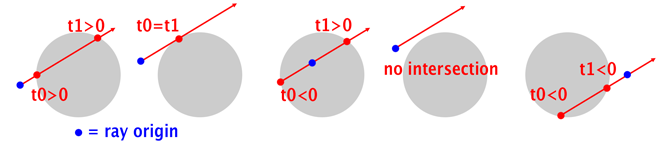
When \(\Delta > 0\), there are two roots, which can be calculated with:$$ \dfrac{-b + \sqrt{\Delta}}{2a} \quad \text{and} \quad \dfrac{-b - \sqrt{\Delta}}{2a} $$ In this case, the ray intersects the sphere at two points (\(t_0\) and \(t_1\)).
-
When \(\Delta = 0\), there is one root, which can be calculated with:$$ -\dfrac{b}{2a} $$ The ray intersects the sphere at one point only (\(t_0 = t_1\)).
-
When \(\Delta < 0\), there is no real solution, indicating that the ray does not intersect the sphere.
Since we have \(a\), \(b\), and \(c\), we can easily solve these equations to find the values for \(t\), which correspond to the two intersection points of the ray with the sphere (\(t_0\) and \(t_1\) in Figure 1). Note that the root values can be negative, meaning that the ray intersects the sphere but is behind the origin. One root can be negative, and the other positive, indicating that the ray's origin is inside the sphere. There might also be no solution to the quadratic equation, meaning that there is no intersection between the ray and the sphere.
Before we explore how to implement this algorithm in C++, let's see how we can solve the same problem when the sphere is not centered at the origin. Then, we can rewrite equation 2 as:
$$ |P-C|^2-R^2=0 $$Where \(C\) is the center of the sphere in 3D space. Equation 4 can now be rewritten as:
$$|O+tD-C|^2-R^2=0.$$This gives us the following:
$$ \begin{array}{l} a = D^2 = 1\\ b = 2D \cdot (O-C)\\ c = |O-C|^2 - R^2 \end{array} $$In a more intuitive form, this means that we can translate the ray by \(-C\) and test this transformed ray against the sphere as if it was centered at the origin.
"Why \(a=1\)"? Because \(D\), the ray's direction, is a vector that is normally normalized. The result of a vector squared is the same as a dot product of the vector with itself. We know that the dot product of a normalized vector with itself is 1, therefore \(a=1\). However, you must be very careful in your code because the rays tested for intersections with a sphere don't always have their direction vector normalized, so you will have to calculate the value for \(a\) (check code further down). This is a pitfall that is often the source of bugs in the code.
Computing the Intersection Point
Once we have the value for \(t_0\), computing the intersection position or hit point is straightforward. We simply apply the ray parametric equation:
$$P_{hit} = O + t_0 D.$$Vec3f Phit = ray.orig + ray.dir * t_0;
Computing the Normal at the Intersection Point
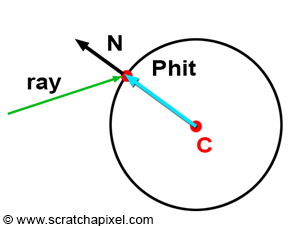
There are various methods to calculate the normal of a point lying on the surface of an implicit shape. However, as mentioned in the first chapter of this lesson, one method involves differential geometry, which is mathematically quite complex. Thus, we will opt for a much simpler approach. For instance, the normal of a point on a sphere can be computed as the position of the point minus the sphere center (it's essential to normalize the resulting vector):
$$N = \frac{P - C}{||P - C||}.$$Vec3f Nhit = normalize(Phit - sphere.center);
Computing the Texture Coordinates at the Intersection Point
Interestingly, texture coordinates are essentially the spherical coordinates of the point on the sphere, remapped to the range [0, 1]. Recalling the previous chapter and the lesson on Geometry, the Cartesian coordinates of a point can be derived from its spherical coordinates as follows:
$$ \begin{array}{l} P.x = \cos(\theta)\sin(\phi),\\ P.y = \sin(\theta),\\ P.z = \cos(\theta)\sin(\phi).\\ \end{array} $$These equations may vary if a different convention is used. The spherical coordinates \(\theta\) and \(\phi\) can also be deduced from the Cartesian coordinates of the point using the following equations:
$$ \begin{array}{l} \phi = \text{atan2}(z, x),\\ \theta = \text{acos}\left(\dfrac{P.y}{R}\right). \end{array} $$Where \(R\) is the radius of the sphere. These equations are further explained in the lesson on Geometry. Sphere coordinates are valuable for texture mapping or procedural texturing. The program in this lesson will demonstrate how they can be utilized to create patterns on the surface of spheres.
Implementing the Ray-Sphere Intersection Test in C++
Let's explore how we can implement the ray-sphere intersection test using the analytic solution. Directly applying equation 5 is feasible (and it will work) to calculate the roots. However, due to the finite precision with which real numbers are represented on computers, this formula can suffer from a loss of significance. This issue arises when \(b\) and the square root of the discriminant have close values but opposite signs. Given the limited precision of floating-point numbers on computers, this can lead to catastrophic cancellation or unacceptable rounding errors. For more details on this issue, plenty of resources are available online. However, equation 5 can be substituted with a slightly modified equation that proves to be more stable in computer implementations:
$$ \begin{array}{l} q = -\dfrac{1}{2} \left( b + \text{sign}(b) \sqrt{b^2 - 4ac} \right) \\ x_{1} = \dfrac{q}{a}, \quad x_{2} = \dfrac{c}{q} \end{array} $$Where \(\text{sign}\) is -1 when \(b\) is less than 0, and 1 otherwise. This modification ensures that the quantities combined to compute \(q\) share the same sign, thus avoiding catastrophic cancellation. Below is how the routine is implemented in C++:
bool solveQuadratic(const float &a, const float &b, const float &c,
					float &x0, float &x1) {
    float discr = b * b - 4 * a * c;
    if (discr < 0) return false;
    else if (discr == 0) x0 = x1 = -0.5 * b / a;
    else {
        float q = (b > 0) ?
            -0.5 * (b + sqrt(discr)) :
            -0.5 * (b - sqrt(discr));
        x0 = q / a;
        x1 = c / q;
    }
    if (x0 > x1) std::swap(x0, x1);

    return true;
}
Now, here is the complete code for the ray-sphere intersection test. For the geometric solution, we noted that we could reject the ray early if \(d\) is greater than the sphere's radius. However, this would involve computing the square root of \(d^2\), which incurs a computational cost. Moreover, \(d\) itself is never used in the code; only \(d^2\) is. Instead of computing \(d\), we test if \(d^2\) is greater than \(radius^2\) (hence why \(radius^2\) is calculated in the constructor of the Sphere class) and reject the ray if this condition is true. This approach efficiently speeds up the process.
bool intersect(const Ray &ray) const
{
        float t0, t1; // Solutions for t if the ray intersects the sphere
#if 0
        // Geometric solution
        Vec3f L = center - ray.orig;
        float tca = L.dotProduct(ray.dir);
        // if (tca < 0) return false;
        float d2 = L.dotProduct(L) - tca * tca;
        if (d2 > radius * radius) return false;
        float thc = sqrt(radius * radius - d2);
        t0 = tca - thc;
        t1 = tca + thc;
#else
        // Analytic solution
        Vec3f L = ray.orig - center;
        float a = ray.dir.dotProduct(ray.dir);
        float b = 2 * ray.dir.dotProduct(L);
        float c = L.dotProduct(L) - radius * radius;
        if (!solveQuadratic(a, b, c, t0, t1)) return false;
#endif
        if (t0 > t1) std::swap(t0, t1);

        if (t0 < 0) {
            t0 = t1; // If t0 is negative, let's use t1 instead.
            if (t0 < 0) return false; // Both t0 and t1 are negative.
        }

        t = t0;

        return true;
}
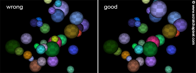
Note: If the scene contains multiple spheres, they are tested in the order they were added to the scene, not necessarily sorted by depth relative to the camera position. The correct approach is to track the sphere with the closest intersection distance, i.e., the smallest \(t\). The image below illustrates a scene render showing the latest intersected sphere in the object list on the left, even if it's not the closest. On the right, the render keeps track of the closest object to the camera, yielding the correct result. The implementation of this technique is provided in the next chapter.
Let's now see how we can implement the ray-sphere intersection test using the analytic solution. We could use equation 5 directly (you can implement it, and it will work) to calculate the roots. Still, on computers, we have a limited capacity to represent real numbers with the precision needed to calculate these roots as accurately as possible. Thus the formula suffers from the effect of a loss of significance. This happens when b and the root of the discriminant don't have the same sign but have values very close to each other. Because of the limited numbers used to represent floating numbers on the computer, in that particular case, the numbers would either cancel out when they shouldn't (this is called catastrophic cancellation) or round off to an unacceptable error (you will easily find more information related to this topic on the internet). However, equation 5 can easily be replaced with a slightly different equation that proves more stable when implemented on computers. We will use instead:
$$ \begin{array}{l} q=-\dfrac{1}{2}(b+sign(b)\sqrt{b^2-4ac})\\ x_{1}=\dfrac{q}{a}\\ x_{2}=\dfrac{c}{q} \end{array} $$Where the sign is -1 when b is lower than 0 and 1 otherwise, this formula ensures that the quantities added for q have the same sign, avoiding catastrophic cancellation. Here is how the routine looks in C++:
bool solveQuadratic(const float &a, const float &b, const float &c, float &x0, float &x1)
{
    float discr = b * b - 4 * a * c;
    if (discr < 0) return false;
    else if (discr == 0) x0 = x1 = - 0.5 * b / a;
    else {
        float q = (b > 0) ?
            -0.5 * (b + sqrt(discr)) :
            -0.5 * (b - sqrt(discr));
        x0 = q / a;
        x1 = c / q;
    }
    if (x0 > x1) std::swap(x0, x1);

    return true;
}
Finally, here is the completed code for the ray-sphere intersection test. For the geometric solution, we have mentioned that we can reject the ray early on if \(d\) is greater than the sphere radius. However, that would require computing the square root of \(d^2\), which has a cost. Furthermore, \(d\) is never used in the code. Only \(d^2\) is. Instead of computing \(d\), we test if \(d^2\) is greater than \(radius^2\) (which is the reason why we calculate \(radius^2\) in the constructor of the Sphere class) and reject the ray if this test is true. It is a simple way of speeding things up.
bool intersect(const Ray &ray) const
{
        float t0, t1; // solutions for t if the ray intersects
#if 0
        // Geometric solution
        Vec3f L = center - ray.orig;
        float tca = L.dotProduct(ray.dir);
        // if (tca < 0) return false;
        float d2 = L.dotProduct(L) - tca * tca;
        if (d2 > radius * radius) return false;
        float thc = sqrt(radius * radius - d2);
        t0 = tca - thc;
        t1 = tca + thc;
#else
        // Analytic solution
        Vec3f L = ray.orig - center;
        float a = ray.dir.dotProduct(ray.dir);
        float b = 2 * ray.dir.dotProduct(L);
        float c = L.dotProduct(L) - radius * radius;
        if (!solveQuadratic(a, b, c, t0, t1)) return false;
#endif
        if (t0 > t1) std::swap(t0, t1);

        if (t0 < 0) {
            t0 = t1; // If t0 is negative, let's use t1 instead.
            if (t0 < 0) return false; // Both t0 and t1 are negative.
        }

        t = t0;

        return true;
}
Note that if the scene contains more than one sphere, the spheres are tested for any given ray in the order they were added to the scene. The spheres are thus unlikely to be sorted in depth (with respect to the camera position). The solution to this problem is to keep track of the sphere with the closest intersection distance, in other words, with the closest \(t\). In the image below, you can see on the left a render of the scene in which we display the latest sphere in the object list that the ray intersected (even if it is not the closest object). On the right, we keep track of the object with the closest distance to the camera and only display this object in the final image, which gives us the correct result. An implementation of this technique is provided in the next chapter.