An Overview of the Rasterization Algorithm
Reading time: 20 mins.Everything You Wanted to Know About the Rasterization Algorithm (But Were Afraid to Ask!)
The rasterization rendering technique is undoubtedly the most commonly used technique for rendering images of 3D scenes. Yet, it is probably the least understood and the least properly documented technique of all, especially when compared to ray tracing.
The reasons for this are multifaceted. Firstly, it's a technique from the past. This is not to suggest that the technique is obsolete—quite the contrary. Most of the techniques used to produce an image with this algorithm were developed between the 1960s and the early 1980s. In the realm of computer graphics, this period is akin to the middle ages, and the knowledge of the papers in which these techniques were developed tends to be lost. Rasterization is also the technique used by GPUs to produce 3D graphics. Although hardware technology has significantly evolved since GPUs were first invented, the fundamental techniques they implement to produce images have not changed much since the early 1980s. The hardware has evolved, but the underlying pipeline by which an image is formed has not. In fact, these techniques are so fundamental and so deeply integrated within the hardware architecture that they often go unnoticed (only people designing GPUs truly understand what they do, and this is far from being a trivial task. However, designing a GPU and understanding the principle of the rasterization algorithm are two distinct challenges; thus, explaining the latter should not be as difficult!).
Regardless, we thought it urgent and important to address this situation. With this lesson, we aim to be the first resource that provides a clear and complete overview of the algorithm, as well as a full practical implementation of the technique. If this lesson has provided the answers you've been desperately seeking, please consider making a donation! This work is provided for free and requires many hours of hard work.
Note: This lesson was published sometime in the mid-2010s.
Introduction
Rasterization and ray tracing both aim to solve the visibility or hidden surface problem, albeit in different orders (the visibility problem was introduced in the lesson Rendering an Image of a 3D Scene, an Overview). What these algorithms have in common is their fundamental use of geometric techniques to address this issue. In this lesson, we will briefly describe how the rasterization algorithm works. Understanding the principle is quite straightforward, but implementing it requires the use of a series of techniques, notably from the field of geometry, which are also explained in this lesson.
The program we develop in this lesson to demonstrate rasterization in practice is significant because we will use it again in subsequent lessons to implement the ray-tracing algorithm. Having both algorithms implemented within the same program will enable us to easily compare the output produced by the two rendering techniques (they should both yield the same result, at least before shading is applied) and assess their performance. This comparison will be an excellent way to better understand the advantages and disadvantages of each algorithm.
The Rasterization Algorithm
There are multiple rasterization algorithms, but to get straight to the point, let's say that all these different algorithms are based on the same overarching principle. In other words, these algorithms are variants of the same idea. It is this idea or principle we will refer to when we discuss rasterization in this lesson.
What is that idea? In previous lessons, we discussed the difference between rasterization and ray tracing. We also suggested that the rendering process could essentially be decomposed into two main tasks: visibility and shading. Rasterization, to put it briefly, is primarily a method to solve the visibility problem. Visibility involves determining which parts of 3D objects are visible to the camera. Some parts of these objects may be hidden because they are either outside the camera's field of view or obscured by other objects.
This problem can be addressed in essentially two ways. One approach is to trace a ray through every pixel in the image to determine the distance between the camera and any intersected object (if any). The object visible through that pixel is the one with the smallest intersection distance (generally denoted as \(t\)). This technique is employed in ray tracing. In this case, an image is created by looping over all pixels in the image, tracing a ray for each, and determining if these rays intersect any objects in the scene. In essence, the algorithm requires two main loops. The outer loop iterates over the pixels in the image, and the inner loop iterates over the objects in the scene:
for (each pixel in the image) {
    Ray R = computeRayPassingThroughPixel(x,y);
    float tClosest = INFINITY;
    Triangle triangleClosest = NULL;
    for (each triangle in the scene) {
        float tHit;
        if (intersect(R, object, tHit)) {
             if (tHit < tClosest) {
                 tClosest = tHit;
                 triangleClosest = triangle;
             }
        }
    }
    if (triangleClosest) {
        imageAtPixel(x,y) = triangleColorAtHitPoint(triangleClosest, tClosest);
    }
}
Note that in this example, objects are assumed to be composed of triangles (and triangles only). Instead of iterating over objects, we consider the objects as a collection of triangles and iterate over these triangles. For reasons already explained in previous lessons, the triangle is often used as the basic rendering primitive in both ray tracing and rasterization (GPUs require geometry to be triangulated).
Ray tracing represents the first approach to solving the visibility problem. We describe the technique as image-centric because rays are shot from the camera into the scene (starting from the image), as opposed to the other approach, which is used in rasterization.

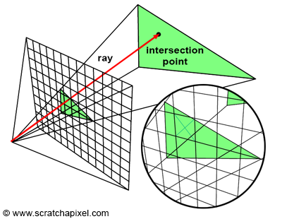
Rasterization adopts the opposite approach to solve the visibility problem. It "projects" triangles onto the screen, converting a 3D representation into a 2D representation of that triangle using perspective projection. This transformation is achieved by projecting the vertices that compose the triangle onto the screen (using perspective projection, as explained). The subsequent step in the algorithm involves employing a technique to fill all the image pixels covered by that 2D triangle. These two steps are depicted in Figure 2. Technically, they are straightforward to execute. The projection steps merely necessitate a perspective divide and a remapping of the resultant coordinates from image space to raster space, processes we've already explored in previous lessons. Determining which pixels in the image are covered by the resulting triangles is equally simple and will be detailed later.
How does this algorithm compare to the ray tracing approach? Firstly, unlike iterating over all pixels in the image first, in rasterization, the outer loop requires iterating over all the triangles in the scene. Then, in the inner loop, we iterate over all pixels in the image to ascertain if the current pixel falls within the "projected image" of the current triangle (as shown in Figure 2). In essence, the inner and outer loops of the two algorithms are reversed.
// Rasterization algorithm
for (each triangle in the scene) {
    // STEP 1: Project vertices of the triangle using perspective projection
    Vec2f v0 = perspectiveProject(triangle[i].v0);
    Vec2f v1 = perspectiveProject(triangle[i].v1);
    Vec2f v2 = perspectiveProject(triangle[i].v2);
    for (each pixel in the image) {
        // STEP 2: Determine if this pixel is contained within the projected image of the triangle
        if (pixelContainedIn2DTriangle(v0, v1, v2, x, y)) {
            image(x, y) = triangle[i].color;
        }
    }
}
This algorithm is object-centric because it starts with the geometry and works its way back to the image, as opposed to the ray tracing approach, which begins with the image and works its way into the scene.
Both algorithms are straightforward in principle, but they diverge slightly in complexity when it comes to implementation and solving the various problems they encounter. In ray tracing, generating the rays is simple, but finding the ray's intersection with geometry can be challenging (depending on the geometry type) and potentially computationally intensive. However, let's set ray tracing aside for now. In the rasterization algorithm, we need to project vertices onto the screen, which is simple and quick. We'll see that the second step, determining if a pixel is contained within the 2D representation of a triangle, has an equally straightforward geometric solution. In essence, computing an image using the rasterization approach relies on two very simple and fast techniques: the perspective process and determining if a pixel lies within a 2D triangle. Rasterization exemplifies an "elegant" algorithm. The techniques it employs are simple to solve; they're also easy to implement and yield predictable results. For all these reasons, the algorithm is ideally suited for GPUs and is the rendering technique used by GPUs to generate images of 3D objects (it can also be easily run in parallel).
In summary:
-
Converting geometry to triangles simplifies the process. If all primitives are converted to the triangle primitive, we can develop fast and efficient functions to project triangles onto the screen and determine if pixels fall within these 2D triangles.
-
Rasterization is object-centric. We project geometry onto the screen and ascertain their visibility by looping over all pixels in the image.
-
It primarily relies on two techniques: projecting vertices onto the screen and determining if a specific pixel lies within a 2D triangle.
-
The rendering pipeline run on GPUs is based on the rasterization algorithm.
"The fast rendering of 3D Z-buffered linearly interpolated polygons is fundamental to state-of-the-art workstations. In general, the problem consists of two parts: 1) the 3D transformation, projection, and light calculation of the vertices, and 2) the rasterization of the polygon into a frame buffer." (A Parallel Algorithm for Polygon Rasterization, Juan Pineda - 1988)
The term rasterization originates from the fact that polygons (triangles in this case) are broken down, in a manner of speaking, into pixels, and as we know, an image composed of pixels is called a raster image. This process is technically known as the rasterization of triangles into an image or frame buffer.
"Rasterization is the process of determining which pixels are inside a triangle, and nothing more." (Michael Abrash in Rasterization on Larrabee)
By this point in the lesson, you should understand how the image of a 3D scene (composed of triangles) is generated using the rasterization approach. What we've described so far is the algorithm's simplest form. It can be significantly optimized, and furthermore, we haven't yet explained what occurs when two triangles projected onto the screen overlap the same pixels in the image. When that happens, how do we decide which of these two (or more) triangles is visible to the camera? We will now address these two questions.
What happens if my geometry is not made of triangles? Can I still use the rasterization algorithm? The simplest solution to this problem is to triangulate the geometry. Modern GPUs only render triangles (as well as lines and points), so you are required to triangulate the geometry anyway. Rendering 3D geometry introduces a series of problems that can be more easily solved with triangles. You will understand why as we progress through the lesson.
Optimizing the Rasterization Process: Utilizing 2D Triangle Bounding Boxes
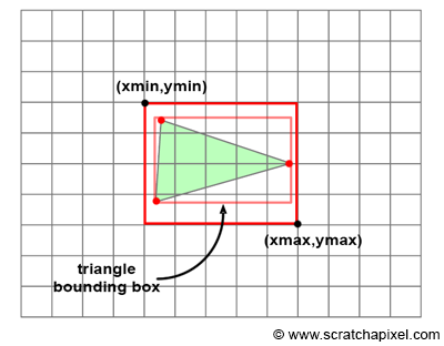
The issue with the naive implementation of the rasterization algorithm we have discussed so far is that it necessitates iterating over all pixels in the image within the inner loop, even though only a small fraction of these pixels may be encompassed by the triangle (as depicted in Figure 3). Of course, this is contingent on the triangle's size on the screen. But considering that we aim to render not just one triangle but an object composed of potentially hundreds to millions of triangles, it's improbable that these triangles will occupy a large area of the image in a typical production example.
There are various methods to reduce the number of pixels tested, but the most common involves computing the 2D bounding box of the projected triangle and iterating over the pixels within this 2D bounding box instead of the entire image. While some pixels might still fall outside the triangle, this approach can significantly enhance the algorithm's performance on average, as illustrated in Figure 3.
Computing the 2D bounding box of a triangle is straightforward. We need to identify the minimum and maximum x and y coordinates of the triangle's vertices in raster space. The following pseudo code illustrates this process:
// Convert the vertices of the current triangle to raster space
Vec2f bbmin = INFINITY, bbmax = -INFINITY;
Vec2f vproj[3];
for (int i = 0; i < 3; ++i) {
    vproj[i] = projectAndConvertToNDC(triangle[i].v[i]);
    // Coordinates are in raster space but still floats, not integers
    vproj[i].x *= imageWidth;
    vproj[i].y *= imageHeight;
    if (vproj[i].x < bbmin.x) bbmin.x = vproj[i].x;
    if (vproj[i].y < bbmin.y) bbmin.y = vproj[i].y;
    if (vproj[i].x > bbmax.x) bbmax.x = vproj[i].x;
    if (vproj[i].y > bbmax.y) bbmax.y = vproj[i].y;
}
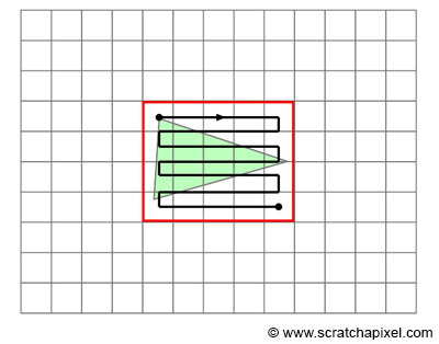
After calculating the 2D bounding box of the triangle (in raster space), we merely need to iterate over the pixels defined by that box. However, it's crucial to be mindful of how raster coordinates, defined as floats in our code, are converted to integers. Notably, one or two vertices might be projected outside the canvas boundaries, meaning their raster coordinates could be less than 0 or exceed the image size. We address this issue by clamping the pixel coordinates within the range [0, Image Width - 1] for the x coordinate, and [0, Image Height - 1] for the y coordinate. Additionally, we must round the bounding box's minimum and maximum coordinates to the nearest integer value (this approach is effective when iterating over the pixels in the loop because we initialize the variable to xmin or ymin and exit the loop when the variable x or y exceeds xmax or ymax). All these adjustments should be made before employing the final fixed-point (or integer) bounding box coordinates in the loop. Here's the pseudo-code:
...
uint xmin = std::max(0, std::min(imageWidth - 1, std::floor(bbmin.x)));
uint ymin = std::max(0, std::min(imageHeight - 1, std::floor(bbmin.y)));
uint xmax = std::max(0, std::min(imageWidth - 1, std::floor(bbmax.x)));
uint ymax = std::max(0, std::min(imageHeight - 1, std::floor(bbmax.y)));
for (y = ymin; y <= ymax; ++y) {
    for (x = xmin; x <= xmax; ++x) {
        // Check if the current pixel lies within the triangle
        if (pixelContainedIn2DTriangle(v0, v1, v2, x, y)) {
            image(x,y) = triangle[i].color;
        }
    }
}
Note that production rasterizers utilize methods more efficient than looping over the pixels contained within a triangle's bounding box. As mentioned, many pixels do not overlap with the triangle, and testing these pixel samples for overlap is inefficient. These more optimized methods are beyond the scope of this lesson.
If you have studied this algorithm or how GPUs render images, you might have heard or read that the coordinates of projected vertices are sometimes converted from floating point to fixed point numbers (in other words, integers). The rationale for this conversion is that basic operations such as multiplication, division, addition, etc., on fixed point numbers can be executed very quickly (compared to the time required to perform the same operations with floating point numbers). While this was commonly the case in the past, and GPUs are still designed to work with integers at the rasterization stage of the rendering pipeline, modern CPUs generally include FPUs (floating-point units). Therefore, if your program is running on the CPU, there is likely little to no benefit in using fixed point numbers (in fact, it might even run slower).
Understanding the Image Buffer and Frame Buffer
Our objective is to produce an image of the scene. We have two methods for visualizing the result of the program: either by displaying the rendered image directly on the screen or by saving the image to disk to view it later with a program such as Photoshop. However, in both scenarios, we need a way to store the image that is being rendered while it is in the process of rendering. For this purpose, we utilize what is referred to in computer graphics as an image or frame-buffer. This is simply a two-dimensional array of colors matching the size of the image. Before the rendering process begins, the frame-buffer is created, and all pixels are initially set to black. During rendering, as triangles are rasterized, if a given pixel overlaps a triangle, then the color of that triangle is stored in the frame-buffer at the corresponding pixel location. Once all triangles have been rasterized, the frame-buffer will contain the complete image of the scene. The final step is to either display the content of the buffer on the screen or save it to a file. In this lesson, we will opt for the latter.
Unfortunately, there is no cross-platform solution for displaying images directly on the screen, which is regrettable. For this reason, it is more practical to save the content of the image to a file and use a cross-platform application such as Photoshop or another image editing tool to view the image. The software you use to view the image must naturally support the format in which the image is saved. In this lesson, we will employ the simple PPM image file format.
However, we have just released a lesson in section 2 of this website on how to display images on the screen. For now, we have an example for users of the Windows OS, with support for Mac and Linux coming soon. So, if you are interested in learning how to display the result of your program directly on the screen, have a look at this lesson. Otherwise, you can save the result to a file as suggested above and view the result in a paint program such as Gimp or Photoshop.
Resolving Overlaps with the Depth Buffer: Handling Multiple Triangles per Pixel
Keep in mind, the primary goal of the rasterization algorithm is to resolve the visibility issue. To accurately display 3D objects, identifying which surfaces are visible is crucial. In the early days of computer graphics, two methods were prevalent for addressing the "hidden surface" problem (another term for the visibility issue): the Newell algorithm and the z-buffer. We mention the Newell algorithm only for historical context and will not cover it in this lesson, as it is no longer in use. Our focus will be solely on the z-buffer method, which remains a standard approach in GPU technology.
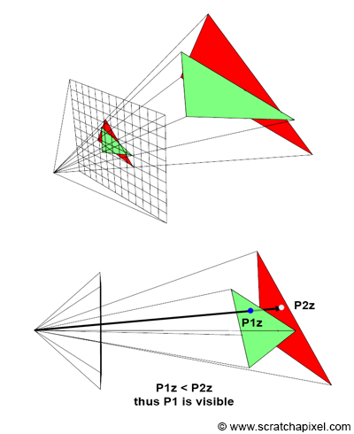
Yet, to operationalize a basic rasterizer, we must consider that more than one triangle may cover the same pixel in the image (as depicted in Figure 5). How, then, do we determine which triangle is visible? The solution is straightforward: employ a z-buffer, also known as a depth buffer, a term you've likely encountered. A z-buffer is essentially another two-dimensional array, matching the image's dimensions. Unlike the array of colors, it consists of floating-point numbers. Before rendering begins, each pixel in this array is initialized to a very large number. When a pixel overlaps a triangle, we also check the value in the z-buffer at that pixel's location. This array records the distance from the camera to the nearest overlapped triangle for each pixel. Since this initial value is set to infinity (or any significantly large number), the first detected overlap of pixel X with triangle T1 will undoubtedly be closer than the value in the z-buffer. We then update that pixel's value with the distance to T1. If the same pixel X later overlaps another triangle T2, we compare this new triangle's distance to the camera against the z-buffer's stored value (now reflecting the distance to T1). If T2 is closer, it obscures T1; otherwise, T1 remains the closest encountered triangle for that pixel. Thus, we either update the z-buffer with T2's distance or maintain T1's distance if it remains the closest. The z-buffer, therefore, records the nearest object's distance for each pixel in the scene (though we'll delve into the specifics of "distance" later in this lesson). In Figure 5, the red triangle is positioned behind the green triangle in three-dimensional space. If we render the red before the green triangle, for any pixel covering both, we initially set, then update the z-buffer with the distances to the red and subsequently the green triangle.
You might wonder how we ascertain the distance from the camera to a triangle. Let's first examine an implementation of this algorithm in pseudo-code, and we'll revisit this question later (for now, let's assume the function pixelContainedIn2DTriangle calculates this distance for us):
// A z-buffer is merely a 2D array of floats
float buffer = new float[imageWidth * imageHeight];
// Initialize the distance for each pixel to a significantly large number
for (uint32_t i = 0; i < imageWidth * imageHeight; ++i)
    buffer[i] = INFINITY;

for (each triangle in the scene) {
    // Project vertices
    ...
    // Compute bbox of the projected triangle
    ...
    for (y = ymin; y <= ymax; ++y) {
        for (x = xmin; x <= xmax; ++x) {
            // Check if the current pixel is within the triangle
            float z;  // Distance from the camera to the triangle
            if (pixelContainedIn2DTriangle(v0, v1, v2, x, y, &z)) {
                // If the distance to that triangle is shorter than what's stored in the
                // z-buffer, update the z-buffer and the image at pixel location (x,y)
                // with the color of that triangle
                if (z < zbuffer(x, y)) {
                    zbuffer(x, y) = z;
                    image(x, y) = triangle[i].color;
                }
            }
        }
    }
}
Looking Ahead: Further Explorations in Rasterization
This is only a very high-level overview of the algorithm (as illustrated in Figure 6), but it should give you a good idea of what components are necessary in the program to produce an image. We will need:
-
An image buffer (a 2D array of colors),
-
A depth buffer (a 2D array of floats),
-
Triangles (the geometry that makes up the scene),
-
A function to project the vertices of the triangles onto the canvas,
-
A function to rasterize the projected triangles,
-
Some code to save the content of the image buffer to disk.

In the next chapter, we will explore how coordinates are converted from camera to raster space. Although the method is identical to the one we studied and presented in the previous lesson, we will introduce a few additional tricks along the way. In Chapter Three, we will learn how to rasterize triangles. Chapter Four will provide a detailed examination of how the z-buffer algorithm functions. As usual, we will conclude this lesson with a practical example.