Rendering an Image of a 3D Scene

The Visibility Problem

Reading time: 21 mins.

The Visibility Problem

We have previously explained the visibility problem. To create a photorealistic image, it's essential to determine which parts of an object are visible from a specific viewpoint. The issue arises when we project the corners of a box, for example, and connect the projected points to draw the edges of the box. As a result, all faces of the box become visible. However, in reality, only the front faces should be visible, with the rear ones hidden.

In computer graphics, this problem is primarily solved using two methods: ray tracing and rasterization. Let's briefly explain how each works. While it's challenging to ascertain which method predates the other, rasterization was significantly more popular in the early days of computer graphics. Ray tracing, known for its higher computational and memory demands, is comparatively slower than rasterization. Given the limited processing power and memory of early computers, rendering images with ray tracing was not deemed feasible for production environments (e.g., film production). Consequently, nearly every renderer utilized rasterization, with ray tracing mostly confined to research projects. However, ray tracing excels over rasterization in simulating effects like reflections, soft shadows, etc., making it easier to produce photorealistic images, albeit at a slower pace. This superiority in simulating realistic shading and light effects will be discussed further in the next chapter. Real-time rendering APIs and GPUs generally favor rasterization due to the premium placed on speed for real-time applications. However, the limitations once faced by ray tracing in the '80s and '90s no longer apply. Modern computers' formidable power means that ray tracing is now employed by virtually all offline renderers today, often in a hybrid approach alongside rasterization. This is primarily because ray tracing is the most straightforward method for simulating critical effects such as sharp and glossy reflections, soft shadows, etc. As long as speed is not a critical factor, it offers numerous advantages over rasterization, though making ray tracing efficient still requires considerable effort.

Pixar's PhotoRealistic RenderMan, the renderer developed by Pixar for its early feature films (Toy Story, Finding Nemo, A Bug's Life), initially utilized a rasterization algorithm. This algorithm, known as REYES (Renders Everything You Ever Saw), is considered one of the most sophisticated visible surface determination algorithms ever devised. The GPU rendering pipeline shares many similarities with REYES. However, Pixar's current renderer, RIS, is a pure ray tracer. The introduction of ray tracing has significantly enhanced the realism and complexity of the images produced by the studio over the years.

Rasterization to Solve the Visibility Problem: How Does it Work?

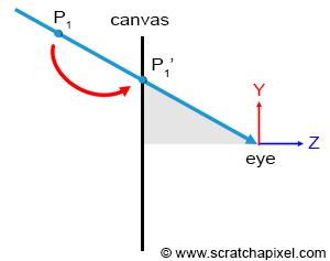
We have already explained the difference between rasterization and ray tracing (refer to the previous chapter). However, let's reiterate that the rasterization approach can be intuitively understood as moving a point along a line that connects \(P\), a point on the geometry's surface, to the eye until it "lies" on the canvas surface. This line is only implicit; we never actually need to construct it, but this is how we can intuitively interpret the projection process.

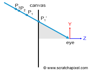
**Figure 1:** The projection process can be visualized as moving the point we want to project down along a line connecting the point or the vertex itself to the eye. We stop moving the point along that line when it lies on the plane of the canvas. Obviously, we don't "slide" the point along this line explicitly, but this is how the projection process can be interpreted.

**Figure 2:** Several points in the scene may project to the same point on the canvas. The point visible to the camera is the one closest to the eye along the ray on which all points are aligned.

The essence of the visibility problem is that situations may arise where several points in the scene, \(P\), \(P1\), \(P2\), etc., project onto the same point \(P'\) on the canvas (recall that the canvas also serves as the screen's surface). However, the only point visible through the camera is the one along the line connecting the eye to all these points, which is closest to the eye, as illustrated in Figure 2.

To solve the visibility problem, we first need to express \(P'\) in terms of its position in the image: what are the pixel coordinates in the image where \(P'\) falls? Remember, projecting a point onto the canvas surface yields another point \(P'\) whose coordinates are real. However, \(P'\) also necessarily falls within a specific pixel of our final image. So, how do we transition from expressing \(P's\) in terms of their position on the canvas surface to defining them in terms of their position in the final image (the pixel coordinates in the image where \(P'\) falls)? This transition involves a simple change of coordinate systems.

The original coordinate system, where the point is defined, is called screen space (or image space). It has an origin located at the canvas center, with all axes of this two-dimensional system having a unit length. The \(x\) or \(y\) coordinate of any point in this system can be negative if it lies to the left of the \(x\)-axis or below the \(y\)-axis.
The raster space is the coordinate system where points are defined with respect to the pixel grid of the image. Its origin is usually at the upper-left corner of the image, with axes also having unit lengths, and a pixel considered as one unit. The actual size of the canvas in this system is given by the image's vertical (height) and horizontal (width) dimensions, expressed in pixels.

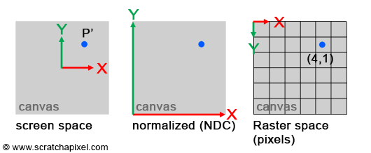
**Figure 3:** Computing the coordinates of a point on the canvas in pixel values requires transforming the points' coordinates from screen to NDC space, and from NDC space to raster space.

Converting points from screen space to raster space is straightforward. Since \(P'\) coordinates in raster space can only be positive, we first normalize \(P's\) original coordinates, converting them from their original range to [0, 1] (such points are defined in NDC space, where NDC stands for Normalized Device Coordinates). After converting to NDC space, transforming the point's coordinates to raster space is straightforward: multiply the normalized coordinates by the image dimensions, then round off the number to the nearest integer value (pixel coordinates must be integers). The original range of \(P'\) coordinates depends on the canvas size in screen space. For simplicity, let's assume the canvas is two units long in each dimension (width and height), meaning \(P'\) coordinates in screen space are within the range \([-1, 1]\). Here is the pseudocode to convert \(P's\) coordinates from screen space to raster space:

int width = 64, height = 64;  // Dimension of the image in pixels 
Vec3f P = Vec3f(-1, 2, 10); 
Vec2f P_proj; 
P_proj.x = P.x / P.z;  //-0.1 
P_proj.y = P.y / P.z;  //0.2 
// Convert from screen space coordinates

 to normalized coordinates
Vec2f P_proj_nor; 
P_proj_nor.x = (P_proj.x + 1) / 2;  //(-0.1 + 1) / 2 = 0.45 
P_proj_nor.y = (1 - P_proj.y) / 2;  //(1 - 0.2) / 2 = 0.4 
// Finally, convert to raster space
Vec2i P_proj_raster; 
P_proj_raster.x = (int)(P_proj_nor.x * width); 
P_proj_raster.y = (int)(P_proj_nor.y * height); 
if (P_proj_raster.x == width) P_proj_raster.x = width - 1; 
if (P_proj_raster.y == height) P_proj_raster.y = height - 1;

This content builds on the previous explanation and emphasizes the practical aspects of implementing visibility determination in computer graphics. Here's a revised version with grammar corrections and Markdown formatting:

This conversion process is elaborated in the lesson 3D Viewing: The Pinhole Camera Model.

A few key points should be noted in this code. Firstly, the original point \(P\), the projected point in screen space, and NDC space all utilize the Vec3f or Vec2f types, wherein the coordinates are defined as real numbers (floats). However, the final point in raster space uses the Vec2i type, where coordinates are integers (representing pixel coordinates in the image). Programming arrays are 0-indexed, meaning the coordinates of a point in raster space should never exceed the image width minus one or the image height minus one. This situation may occur when \(P's\) coordinates in screen space are exactly 1 in either dimension. The code addresses this case (lines 14-15), clamping the coordinates to the appropriate range if necessary. Additionally, the origin of the NDC space is located in the lower-left corner of the image, whereas the origin of the raster space system is in the upper-left corner (refer to Figure 3). Thus, the \(y\) coordinate needs to be inverted when converting from NDC to raster space (note the adjustment between lines 8 and 9 in the code).

Why is this conversion necessary? To solve the visibility problem, we employ the following method:

Project all points onto the screen.
- For each projected point, convert \(P's\) coordinates from screen space to raster space.
- Determine the pixel to which the point maps (using the point's raster coordinates) and store the distance from that point to the eye in a special list (the depth list) maintained for that pixel.
"You say, project all points onto the screen. How do we find these points in the first place?"

Indeed, a valid question. Technically, we decompose the triangles or polygons that objects are made of into smaller geometry elements—no larger than a pixel when projected onto the screen. In real-time APIs (OpenGL, DirectX, Vulkan, Metal, etc.), these are often referred to as fragments. For a more detailed explanation, refer to the lesson on the REYES algorithm in this section.
At the process's end, sort the points in each pixel's list in order of increasing distance. As a result, the point visible for any given pixel in the image is the first point from that pixel's list.

"Why do points need to be sorted according to their depth?"

The list needs to be sorted because points are not necessarily ordered by depth when projected onto the screen. If points are inserted by adding them at the top of the list, it's possible to project a point \(B\) that is further from the eye than a point \(A\) after \(A\) has been projected. In such cases, \(B\) would be the first point in the list, despite being further from the eye than \(A\), necessitating sorting.

An algorithm based on this method is called a depth sorting algorithm—a self-explanatory term. The concept of depth ordering is fundamental to all rasterization algorithms. Among the most renowned are:

The z-buffering algorithm, probably the most widely used in this category. The REYES algorithm, presented in this section, implements the z-buffer algorithm. It closely resembles the technique we described, where points on the surfaces of objects (which are subdivided into very small surfaces or fragments) are projected onto the screen and stored in depth lists.
The Painter algorithm
Newell's algorithm
... (this list can be extended)

Keep in mind that although this may sound old-fashioned to you, all graphics cards use at least one implementation of the z-buffer algorithm to produce images. These algorithms, especially z-buffering, are still commonly used today.

Why do we need to keep a list of points?

Storing the point with the shortest distance to the eye doesn't necessarily require storing all the points in a list. Indeed, you could do the following:

For each pixel in the image, set the variable \(z\) to infinity.
For each point in the scene:
- Project the point and compute its raster coordinates.
- If the distance from the current point to the eye, \(z'\), is smaller than the distance \(z\) stored in the pixel the point projects to, then update \(z\) with \(z'\). If \(z'\) is greater than \(z\), then the point is located further away than the point currently stored for that pixel.

This shows that you can achieve the same result without having to store a list of visible points and sorting them out at the end. So, why did we use one? We used one because, in our example, we assumed that all points in the scene were opaque. But what happens if they are not fully opaque? If several semi-transparent points project onto the same pixel, they may be visible through each other. In this case, it is necessary to keep track of all the points visible through that particular pixel, sort them by distance, and use a special compositing technique (which we will learn about in the lesson on the REYES algorithm) to blend them correctly.

Ray Tracing to Solve the Visibility Problem: How Does It Work?

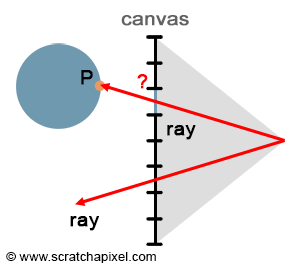
**Figure 4:** In ray tracing, we explicitly trace rays from the eye into the scene. If the ray intersects some geometry, the pixel the ray passes through takes the color of the intersected object.

With rasterization, points are projected onto the screen to find their respective positions on the image plane. However, we can approach the problem from the opposite direction. Rather than going from the point to the pixel, we start with the pixel and convert it into a point on the image plane (taking the center of the pixel and converting its coordinates from raster space to screen space). This results in \(P'\). We then trace a ray starting from the eye, passing through \(P'\), and extending it down into the scene (assuming \(P'\) is the center of the pixel). If the ray intersects an object, then the intersection point, \(P\), is the point visible through that pixel. In short, ray tracing is a method to solve the point's visibility problem by explicitly tracing rays from the eye into the scene.

Note that, in a way, ray tracing and rasterization reflect each other. They are based on the same principle, but ray tracing goes from the eye to the object, while rasterization goes from the object to the eye. While they both identify which point is visible for any given pixel in the image, implementing them requires solving very different problems. Ray tracing is more complicated because it involves solving the ray-geometry intersection problem. Can we find a way to compute whether a ray intersects a sphere, a cone, or another shape, including NURBS, subdivision surfaces, and implicit surfaces?

Over the years, much research has been devoted to finding efficient ways of computing the intersection of rays with the simplest of all shapes—the triangle—as well as directly ray tracing other types of geometry like NURBS and implicit surfaces. Another approach is to convert all geometry into a single geometry representation before the rendering process begins, allowing the renderer to only test the intersection of rays with this unified representation. Since triangles are an ideal rendering primitive, typically, all geometry is converted to triangle meshes. This means instead of implementing a ray-object intersection test for each geometry type, you only need to test the intersection of rays with triangles, which has many advantages:

First, as suggested earlier, the triangle has many properties that make it a very attractive geometry primitive. It's coplanar, indivisible (unlike faces with four or more vertices, which can create more faces by connecting existing vertices), and can easily be subdivided into more triangles. Additionally, the math for computing the barycentric coordinates of a triangle, which is used in texturing, is simple and robust.
A lot of research has been done to find the best possible ray-triangle intersection test. A good ray-triangle intersection algorithm needs to be fast, memory-efficient, and robust, due to challenges like floating-point arithmetic issues.
From a coding perspective, supporting a single routine is far more advantageous than coding many routines to handle all geometry types. Supporting only triangles simplifies the code significantly and allows for the design of code that works best with triangles in general. This is particularly true when it comes to acceleration structures, which are essential for quickly discarding scene sections that are unlikely to be intersected by the ray and testing only for subsections that the ray might potentially intersect. These strategies save a considerable amount of time and are generally based on acceleration structures. It's worth noting that specially designed hardware has already been built to handle the ray-triangle intersection test specifically, allowing complex scenes to run near real-time using ray tracing. It's quite clear that in the future, graphics cards will natively support the ray-triangle intersection test, and video games will evolve towards ray tracing.

Comparing Rasterization and Ray-Tracing

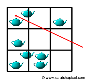
**Figure 5:** The principle of an acceleration structure consists of dividing space into sub-regions. As the ray travels from one sub-region to the next, we only need to check for a possible intersection with the geometry contained in the current sub-region. Instead of testing all the objects in the scene, we can test only those contained in the sub-regions the ray passes through. This leads to potentially saving a lot of ray-geometry intersection tests, which are costly.

We have already discussed the differences between ray tracing and rasterization a few times. Why would you choose one over the other? As mentioned before, for solving the visibility problem, rasterization is faster than ray tracing. Why is that? Converting geometry to make it work with the rasterization algorithm eventually takes some time, but projecting the geometry itself is very fast (it just takes a few multiplications, additions, and divisions). In comparison, computing the intersection of a ray with geometry requires far more instructions and is, therefore, more expensive. The main difficulty with ray tracing is that render time increases linearly with the amount of geometry the scene contains. Because we have to check whether any given ray intersects any of the triangles in the scene, the final cost is then the number of triangles multiplied by the cost of a single ray-triangle intersection test. Hopefully, this problem can be alleviated by the use of an acceleration structure. The idea behind acceleration structures is that space can be divided into subspaces (for instance, you can divide a box containing all the geometry to form a grid - each cell of that grid represents a sub-space of the original box) and that objects can be sorted depending on the sub-space they fall into. This idea is illustrated in Figure 5.

If these sub-spaces are significantly larger than the objects' average size, then it is likely that a subspace will contain more than one object (of course, it all depends on how they are organized in space). Instead of testing all objects in the scene, we can first test if a ray intersects a given subspace (in other words, if it passes through that sub-space). If it does, we can then test if the ray intersects any of the objects it contains; but if it doesn't, we can then skip the ray-intersection test for all these objects. This leads to only testing a subset of the scene's geometry, which saves time.

If acceleration structures can be used to accelerate ray tracing, then isn't ray tracing superior to rasterization? Yes and no. Firstly, it is still generally slower, but using an acceleration structure raises a lot of new problems.

Firstly, building this structure takes time, which means the render can't start until it's built: this generally never takes more than a few seconds, but if you intend to use ray tracing in a real-time application, then these few seconds are already too much (the acceleration structures need to be built for every rendered frame if the geometry changes from frame to frame).
Secondly, an acceleration structure potentially takes a lot of memory. This all depends on the scene complexity; however, because a good chunk of the memory needs to be used for the acceleration structure, this means that less is available for doing other things, particularly storing geometry. In practice, this means you can potentially render less geometry with ray tracing than with rasterization.
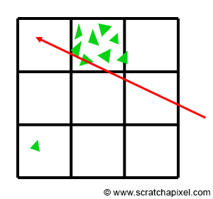
Finally, finding a good acceleration structure is very difficult. Imagine that you have one triangle on one side of the scene and all the other triangles stuck together in a very small region of space. If we build a grid for this scene, many of the cells will be empty, but the main problem is that when a ray traverses the cell containing the cluster of triangles, we will still need to perform a lot of intersection tests. Saving one test over the hundreds that may be required is negligible and clearly shows that a grid as an acceleration structure for that sort of scene is not a good choice. As you can see, the efficiency of the acceleration structure depends very much on the scene and the way objects are scattered: are objects small or large, is it a mix of small and large objects, are objects uniformly distributed over space or very unevenly distributed? Is the scene a combination of any of these options?

Many different acceleration structures have been proposed, and they all have, as you can guess, strengths and weaknesses, but of course, some of them are more popular than others. You will find many lessons devoted to this particular topic in the section devoted to Ray Tracing Techniques.

From reading all this, you may think that all problems are with ray tracing. Well, ray tracing is popular for a reason. Firstly, in its principle, it is incredibly simple to implement. We showed in the first lesson of this section that a very basic raytracer can be written in no more than a few hundred lines of code. In reality, we could argue that it wouldn't take much more code to write a renderer based on the rasterization algorithm, but still, the concept of ray tracing seems to be easier to code, as maybe it is a more natural way of thinking of the process of making an image of a 3D scene. But far more importantly, it happens that if you use ray tracing, computing effects such as reflection or soft shadows, which play a critical role in the photo-realism of an image, are just straightforward to simulate in ray tracing, and very hard to simulate if you use rasterization. To understand why, we first need to look at shading and light transport in more detail, which is the topic of our next chapter.

"Rasterization is fast but needs cleverness to support complex visual effects. Ray tracing supports complex visual effects but needs cleverness to be fast." - David Luebke (NVIDIA).

"With rasterization, it is easy to do it very fast, but hard to make it look good. With ray tracing, it is easy to make it look good, but very hard to make it fast."

Summary

In this chapter, we explored ray tracing and rasterization as two primary methods for solving the visibility problem in 3D rendering. Currently, rasterization is the predominant technique employed by graphics cards to render 3D scenes due to its speed advantage over ray tracing for this specific task. However, ray tracing can be accelerated with the use of acceleration structures, albeit these structures introduce their own challenges. Finding an efficient acceleration structure that performs well irrespective of the scene's complexity, including the number of primitives, their sizes, and their distribution, is difficult. Additionally, acceleration structures demand extra memory, and their construction requires time.

It's crucial to recognize that, at this point, ray tracing does not offer any clear-cut advantages over rasterization in solving the visibility problem. However, ray tracing excels over rasterization in simulating light or shading effects such as soft shadows and reflections. By "excels," we mean that ray tracing facilitates a more straightforward simulation of these effects compared to rasterization. This does not imply that such effects are impossible to achieve with rasterization; rather, they typically require more effort. This clarification is important to counter the common misconception that effects like reflections can only be achieved through ray tracing. This is simply not the case.

Considering the strengths of both techniques, a hybrid approach might be envisioned, where rasterization is used for the initial visibility determination and ray tracing for advanced shading effects in the rendering process. However, integrating both approaches within a single application complicates the development process more than using a unified rendering framework. Given that ray tracing simplifies the simulation of phenomena such as reflections, it often becomes the preferred choice for handling both visibility determination and advanced shading, despite its complexities.