Overview of the Ray-Tracing Rendering Technique

Light Transport Algorithms and Ray-Tracing: Whitted Ray-Tracing

Ray-tracing is one of the most elegant techniques in computer graphics. Many phenomena that are difficult or impossible with other techniques are simple with ray tracing, including shadows, reflections, and refracted light". Robert L. Cook Thomas Porter Loren Carpenter. "Distributed Ray-Tracing" (1984).

Light Transport

As mentioned in the first chapter ray tracing is only a technique used to compute the visibility between points. It is simply a technique based on the concept of a ray which can be mathematically (and in a computer program) defined as a point (the origin of the ray in space) and a direction. Then the idea behind ray-tracing is to find mathematical solutions to compute the intersection of this ray with various types of geometry: triangles, quadrics (which we study in one of the following lessons), NURBs, etc. This is all there is to ray-tracing.

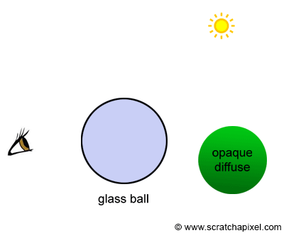
Finding out the color of objects at any point on their surface is a complex problem. The appearance of objects is essentially the result of light bouncing off of the surface of objects or traveling through these objects if they are transparent. Effects like reflection or refraction are the result of light rays being refracted while traveling through transparent surfaces or being reflected off of the surface of a shiny object for example. When we see an object, what we actually "see" are light rays reflected by this object in the direction of our eyes. Many of the rays reflected off of the surface of that object may travel away from the eyes though some of these rays may be indirectly reflected toward the eye by another object in the scene (figure 1). The way light is reflected by objects is a well know and well-studied phenomenon but this is not a lesson on shading, so we won't get into details at this point. All we want you to know in the context of this lesson is that to compute the color of an object at any given point on the surface of that object, we need to simulate the way light is reflected off of the surface of objects. In compute graphics, this is the task of what we call a light transport algorithm. We will study the concept of light transport in detail in some of the following lessons so don't worry too much if only scratch the surface of the subject at this point.

We could simulate the transport of light in the scene in a brute force manner by just applying the laws of optics and physics which describe the way light interacts with matter; we would probably get an extremely accurate image though, the problem with this approach is that (and to stay short) it would probably take a very very long time to get that perfect result, even with some of the most powerful computers we can get today. This approach is simply not practical.

To truly simulate all effects of light accurately, you would have to program the universe.

What light algorithms do is essentially find ways of simulating all sorts of lighting scenarios in an "acceptable" amount of time while providing the best visual accuracy possible. You can see a light transport algorithm as a strategy for solving that light transport problem (and we all know that some strategies to solve a given problem are better than others and that a strategy that is good in a given scenario might not work well in another scenario - light transport algorithms are the same, which is again why so many of them exist).

Computing the new path of a light ray that strikes the surface of an object is something for which we have well-defined mathematic models. The main problem is that the ray may be reflected into the scene and strike the surface of another object in the scene. Thus, if you want to simulate the trajectory or the paths of a light ray as it bounces off from the surface to the surface, what we need is a solution to compute the intersection of rays with surfaces. As you can guess, this is where ray-tracing comes into play. Ray-tracing is of course ideally suited to compute the first visible surface from any given point in the scene in any given direction. Rasterization, in contrast, is not well suited for this task at all. It works well to compute the first visible surface from the camera point of view, but not from any arbitrary point in the scene. Note that it can be done with rasterization. The process would just be very inefficient (readers interested in this approach can search for a technique called hemisphere or hemicube which is used in the radiosity algorithm) even compared to ray-tracing which has a high computational cost.

In conclusion, if these light transport algorithms involve computing the visibility between surfaces, any technique such as ray-tracing or rasterization can be used to do so, though, as explained before, ray-tracing is simply easier to use in this particular context. For this reason, some of the most popular light-transport algorithms such as path-tracing or bidirectional path-tracing have become inevitably associated with ray-tracing. In the end, this has created a confusing situation in which ray-tracing was understood as a technique for creating photo-realistic images. It is not. A photo-realistic computer-generated image is a mix of a light transport algorithm and a technique to compute visibility between surfaces. Thus when you consider any given rendering program, the two questions you may want to ask yourself to understand the characteristics of this particular program are: what light transport algorithm does it use, and what techniques does it use to compute visibility in general: rasterization, ray-tracing or a mix of the two techniques?

As mentioned earlier, don't worry too much about light transport algorithms for now. The point we are trying to make is really that you should not mix ray tracing with the process of actually finding out the color of objects in the scene. We insist on this point as ray tracing is often presented as a technique for producing photo-realistic images of 3D objects. It is not. The job of simulating global illumination effects is that of the light transport algorithm.

For an in-depth introduction to light transport algorithms please read the lesson "Introduction to Shading: The Rendering Equation and Light Transport Algorithms".

Whitted Ray-Tracing

Now that the distinction between ray-tracing and light transport algorithms was established, we can finally introduce one of the most classical examples of light transport algorithms based on ray-tracing. The technique was first detailed in 1980 by Turner Whitted in a Siggraph paper titled "An Improved Illumination Model for Shaded Display". The algorithm is for this reason often given the name of Whitted (-style) ray-tracing.

Before Whitted's paper, most programs were already capable of simulating the look of diffuse and specular surfaces. The famous Phong illumination model (which we will talk about in the lesson devoted to Shaders), was already known. Though, simulating complex reflections and refractions was yet to be done. Whitted proposed to use of ray tracing to solve this problem. If object A is a mirror-like surface, and that object B seats on top of it, then we would like to see the reflection of B into A. If A is not a flat surface, there is no easy solution for computing this reflection. Things get even harder if B is also reflective. Mirror surfaces keep reflecting images of themselves causing the "infinity room" effect which is often seen in films.

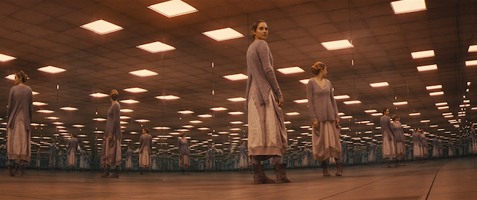
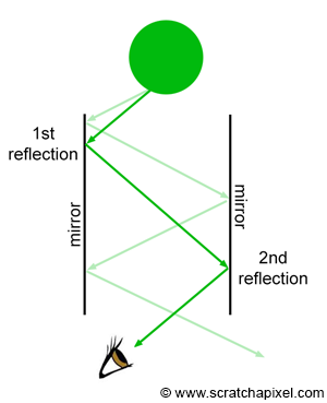
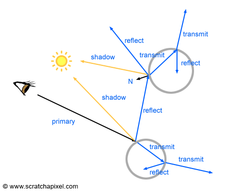
Figure 3 shows an example in which the sphere is reflected a couple of times by the two mirrors before its image finally reaches the eye. What about transparent objects? We should see through transparent surfaces, though materials such as water or glass bend light rays due to the phenomenon of refraction. The optical (and physical) laws governing the phenomena of reflection and refraction are well known. The reflection direction only depends on the surface orientation and the incoming light direction. The refraction direction can be computed using Snell's law and depends on the surface orientation (the surface's normal), the incoming light direction, and the material refractive index (around 1.3 for water and 1.5 for glass). If you know these parameters, computing these directions is just a straight application of the laws of reflection and refractions whose equations are quite simple.

Whitted proposed to use these laws to compute the reflection and refraction direction of rays as they intersect reflective or transparent surfaces, and follow the path of these rays to find out the color of the object they would intersect. Three cases may occur at the intersection point of these reflection and refraction rays (which in CG, we call secondary rays to differentiate them from the primary or camera rays):

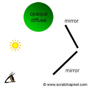
• Case 1: if the surface at the intersection point is opaque and diffuse, all we need to do is use an illumination model such as the Phong model, to compute the color of the object at the intersection point. This process also involves casting a ray in the direction of each light in the scene to find if the point is in shadow. These rays are called shadow rays.

• Case 2: If the surface is a mirror-like surface, we simply trace another reflection ray at the intersection point.

• Case 3: if the surface is transparent, we then cast another reflection and a refraction ray at the intersection point.

If P1 generates a secondary ray that intersects P2 and another secondary ray is generated at P2 that intersects another object at P3, then the color at P3 becomes the color of P2 which in turn becomes the color of P1 (assuming P1 and P2 belong to a mirror-like surface) as shown in Figure 6. The higher the refractive index of a transparent object is, the stronger these specular reflections are. Additionally, the higher the angle of incidence is, the more light is reflected (this is due to the Fresnel effect). The same method is used for refraction rays. If the ray is refracted a P1 then refracted at P2 and then finally hits a diffuse object at P3, P2 takes on the color of P3 and P1 takes on the color of P2 as shown in Figure 7. The higher the refractive index, the stronger the distortion (figure 3).

• Note that Whitted's algorithm uses backward tracing to simulate reflection and refraction, which as mentioned in the previous chapter, is more efficient than forward tracing. We start from the eye, cast primary rays, find the first visible surface and either compute the color of that surface at the intersection point if the object is opaque and diffuse or simply cast a reflection or a reflection and a refraction ray if the surface is either reflective (like a mirror) or transparent.

• Note also that Whitted's algorithm is a light transport algorithm. It can be used to simulate the appearance of diffuse objects (if you use the Phong illumination you would get a mix of diffuse and specular reflection but this is off-topic for now), mirror-like and transparent objects (glass, water, etc.). We will learn how to categorize light transport algorithms based on the sort of lighting effects they can simulate in the introductory lesson on shading [link] (this is very important to see the differences between each algorithm). For example, the Whitted algorithm simulates diffuse and glossy surfaces as well as specular reflection and refraction.

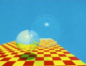
• Finally, and that is probably the most important part, note that Whitted's algorithm relies on computing visibility between points to simulate effects such as reflection, refraction, or shadowing. Once the intersection point P1 is found, we can compute the reflection or refraction direction using the law of reflection or refraction. We then get a new ray direction (or two new directions if the surface is transparent). The next step requires casting this ray into the scene and finding the next intersection point if any (P2 in our examples). And naturally, Whitted used ray-tracing in his particular implementation to compute the visibility between points (between the eye and P1, P1 and P2, P2 and P3, and finally P3 and the light in our examples). On a general note, Whitted was the first to use ray tracing to simulate these effects. Not surprisingly, his technique got a lot of success because it allowed the simulation of physically accurate reflections and refractions for the first time (figure 2).

The Whitted algorithm is the classical example of an algorithm that uses ray tracing to produce photo-realistic computer-generated images. Many more advanced light transport algorithms have been developed since the paper was first published. Let's now review some of the algorithm's properties.

Recursivity

Each time a ray intersects a transparent surface, two new rays are generated (a reflection and a refraction ray). If these rays intersect with another transparent object, each ray will generate two more rays. This process can go on forever, as long as secondary rays keep intersecting reflective or transparent objects. In this particular scenario, the number of rays increases exponentially as the recursion depth increases. The primary ray generates 2 secondary rays. This is the first level of recursion (depth 1). After two levels of recursion (depth 2), 4 rays are generated. At depth 3, each ray produces 2 more rays, thus producing a total of 8 rays. At depth 4, we have 16 rays and at depth 5, 32 rays. This practically means that render time also increases exponentially as the depth increases. The simplest solution to the recursive nature of this algorithm and the fact that the number of secondary rays grows exponentially as the depth increases is to put a cap on the maximum number of allowed recursions (or maximum depth). As soon as the maximum depth is reached, then we simply stop generating new rays.

>, Unlike previous ray tracing algorithms, the visibility calculations do not end when the nearest intersection of a ray with objects in the scene is found. Instead, each visible intersection of a ray with a surface produces more rays in the reflection direction, the refraction direction, and in the direction of each light source. The intersection process is repeated for each ray until none of the new rays intersects any object. "An Improved Illumination Model for Shaded Display", Turner Whitted, 1980

Trees of Rays

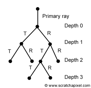
In some papers on ray tracing (especially some of the first papers on the topic), you will often see the term "tree of rays" being used. All the secondary rays spawned by either the primary ray itself or other secondary rays can be represented as a tree as shown in figure 9 (it represents the tree of rays generated by the primary ray in figure 8). Each level in the tree as you go down corresponds to one level of recursion.

To accurately render a two-dimensional image of a three-dimensional scene, global illumination information that affects the intensity of each pixel of the image must be known at the time the intensity is calculated. In a simplified form, this information is stored in a tree of "rays" extending from the viewer to the first surface encountered and from there to other surfaces and to the light sources. "An Improved Illumination Model for Shaded Display", Turner Whitted, 1980.

Implementing Whitted Ray-Tracing in C++

This program provided with this lesson will be different than usual, in the sense that we don't intend to explain it. It uses techniques we haven't studied yet such as the generation of primary rays or the intersection of rays with various types of geometry such as spheres or triangles. The laws of reflection and refraction and the Fresnel equation are used to compute reflections and refractions and the Phong illumination model is used to compute the color of diffuse and glossy objects though again we won't explain how these techniques work in this lesson. You will find them explained one by one in the next lessons.

The main goal of this program is for you to understand the concepts that it is based upon on a higher level. For example, note that the program is essentially structured around the following four main components:

• The main() function in which the scene is created. This involves adding objects and lights to the scene (we just add objects and lights dynamically created to C++ vectors). This is also where the function render() is called.

  int main() 
  { 
   std::vector<Object *> objects; 
   std::vector<Light *> lights; 
   // add objects and lights
   objects.push_back(new Object); 
   ... 
   Options options; 
   options.width = 640; 
   options.height = 480; 
   options.maxDepth = 5; 
   ... 
   render(objects, lights, options); 
   ... 
   return 0; 
  } 
  

• The render() function is the function that loops over all the pixels in the image, generates a primary for each pixel, and casts the resulting primary ray into the scene. Ray-casting itself, the process that involves computing the color of that primary ray, is done by the castRay() function. When all the pixels in the image have been processed, we store the result of the frame buffer in a file. Note that because castRay() is a recursive function we need to keep track of the recursion depth (the variable depth in the castRay() argument list).

  void render(...) 
  { 
   for (j = 0; j < options.height; ++j) { 
    for (i = 0; i < options.width; ++i) { 
  	  // generate primary ray using
  	  ... 
  	  framebuffer[j * options.width + i] = rayCast(orig, dir, objects, lights, options, 0); 
    } 
   } 
  } 
  

• The castRay() function is the function that implements Whitted's light transport algorithm. The ray passed to the function is cast into the scene and the closest visible surface is computed using the trace() function. If the ray intersects an object, we switch between three cases depending on the type of material this object is made of:

  • If the object is transparent, we cast a reflection and a refraction ray. Don't forget to increment the depth value as you call the castRay() function recursively. The resulting colors are mixed using the result of the Fresnel equation (the Fresnel equation returns how much light is reflected based on the incident ray direction, the surface normal, and the material refractive index).

  • If the object is only reflective (like a mirror) we only need to cast a reflection ray.

  • If the object is diffuse and/or glossy we evaluate the Phong illumination model. Shadow rays are cast towards each light in the scene to find if the point is in shadow.

  Note that if the recursion depth is greater than the maximum allowed depth, then the function simply returns the background color and no additional secondary rays are cast.

  Vec3f castRay(const Vec3f &orig, const Vec3f &dir, ..., uint32_t depth)
  {
      if (depth > options.maxDepth)
          return options.backgroundColor;
  
      float tNear = INFINITY;  //distance to the intersected object
      Object *hitObject = NULL;  //pointer to the intersected object
      Vec3f hitColor = 0;  //the color of the intersected point
      if (trace(orig, dir, objects, tnear, hitObject....) {
          switch (hitObject->materialType) {
              case REFLECTION_AND_REFRACTION:
                  // compute reflection and refraction ray
                  ...
                  // cast reflection and refraction ray, don't forget to increment depth
                  Vec3f reflectionColor = castRay(hitPoint, reflectionDirection, ..., depth + 1);
                  Vec3f refractionColor = castRay(hitPoint, refractionDirection, ..., depth + 1);
                  float kr;  //how much light is reflected, computed by the Fresnel equation
                  fresnel(dir, N, hitObject->ior, kr);
                  hitColor = reflectionColor * kr + refractionColor * (1 - kr);
                  break; 
              case REFLECTION:
                  // compute reflection ray
                  ...
                  // cast reflection ray, increment depth
                  Vec3f reflectionColor = castRay(hitPoint, reflectionDirection, ..., depth + 1);
                  hitColor = reflectionColor;
                  break;
              default:
                  // compute Phong illumination model
                  for (uint32_t i = 0; i < lights.size(); ++i) {
                      // compute shadow ray
                      Vec3f lightDirection = lights[i].position - hitPoint;
                      float len2 = dot(lightDirection, lightDirection);  //length^2
                      float tNearShadow = INFINITY;
                      // is hitPoint in the shadow of this light and is the intersection point close to the light itself?
                      bool isInShadow = (trace(hitPoint, normalize(lightDirection), tNearShadow, ...) && tNearShadow * tNearShadow < len2);
                      // compute the Phong model terms
                      hitColor = (1 - isInShadow) * (...);
                  }
                  break;
          }
      }
  
      return hitColor;
  } 
  

• Finally the trace() function itself. It loops over all the objects in the scene and finds the closest surface where the ray intersects. It returns true if the ray intersected an object and false otherwise.

  bool trace(const Vec3f &orig, const Vec3f &dir, float tNear, ...)
  { 
      hitObject = NULL;
      for (uint32_t i = 0; i < objects.size(); ++i) {
          float tNearK = INFINITY;
          if (objects[i]->intersect(orig, dir, tNearK, ...) && tNearK < tNear) {
              hitObject = objects[i];
              tNear = tNearK;
              ...
          }
      }
  
      return (hitObject != NULL);
  }
  

You can find the complete source code of this program in the next chapter. If you compile and run the program, you will probably observe that it takes quite a while to render this simple scene. Here is the output of the program:

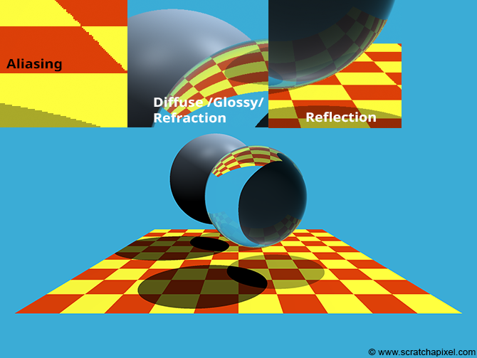
As you can see, we tried to reproduce the image published by Whitted in his original paper. Note though that a few things could be improved in this image. First, if you look at a closeup of the frame itself, you can see that as with rasterization, it suffers from aliasing. We will learn about anti-aliasing techniques for ray tracing in the next lessons. Note also that the shadow under the glass sphere is opaque. This is a case we don't consider, but it would be easy to address it using what we call in ray-tracing the concept of transmission. More on this topic in the next lessons as well.

Is There Anything Better than the Whitted Light-Transport Algorithm?

The method is already a great improvement compared to whatever could be produced before the publication of the paper. Though, certain effects such as glossy reflection (the reflection of objects by glossy surfaces), soft shadows, or caustics can't be simulated with this algorithm. More advanced light-transport algorithms have been developed since then to address these limitations. The most famous ones which are solely based on ray tracing are the path-tracing, the bidirectional path-tracing and Metropolis light transport algorithms. We will study path tracing in this section. Another very important ray-tracing-based algorithm was developed by Robert L. Cook, Thomas Porter, and Loren Carpenter and published in another seminal paper titled "Distributed Ray-Tracing" (1984). We will also study this algorithm in this section.

What's Next?

We are now ready to learn about the foundations of ray tracing. We will learn how to generate primary rays, and intersect rays with simple geometry shapes as well as triangles. From there we will learn how to ray-tracing triangulated meshes, as well as ray-traced objects which have been transformed by a 4x4 affine transformation matrix. We will then have the tools we need to study shading, light-transport algorithms, and effects such as motion blur, depth-of-field, and textures which are all critical to producing photo-realistic computer-generated images.

Exercise

• Add a timer to the program and measure the time it takes to render this simple scene.

• Compute the number of primary, reflection, refraction, and shadow rays that are cast in this scene. Print the numbers out to the terminal at the end of the render.

References

An Improved Illumination Model for Shaded Display. Turner Whitted, 1980