Bézier Curves and Surfaces

Bézier Surfaces

Bézier Surfaces

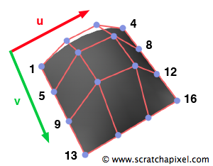
Once we understand the principle of the Bézier curve extending the same technique to the Bézier surface is straightforward. Rather than having 4 points, we will define the surface with 16 points which you can see as a grid of 4x4 control points. We had one parameter to move along the curve (t) for curves. For surfaces, we will need two: one to move in the u direction and one to move in the v direction (see figure 1). Both u and v are contained within the range [0,1]. You can see the process of going from (u, v) to 3D space as a remapping of the unit square (defined by u, v) into a smooth continuous surface within the three-dimensional space. Intuitively, you can see that a Bézier surface is made of many curves going along either the u or v direction. For instance, if we move in the v direction, we need to interpolate the curves defined by points 1, 2, 3, 4 and 5, 6, 7, 8 (and so on for the rest of the surface). If we move along the u direction, the curves defined by points 1, 5, 9, 13, and 2, 6, 10, and 14 need to be interpolated instead. More formally, a point on the Bézier surface depends on the parametric values u and v, and can be defined (equation 1) as a double sum of control points and coefficients ("a sum of Bézier curves"):

whereas for curves,

Is a Bernstein polynomial (equation 2), and

is a binomial coefficient (equation 3). We can see easily see the similarities with curves. If you are interested in the terminology, we say that a Bézier surface (or patch) is constructed as the tensor product of two Bézier curves. Note that we will only consider bicubic Bézier surfaces in this lesson, that is, surfaces for which n = 3 and m = 3. Therefore, the Bernstein polynomials (equation 4) are the same as with bicubic curves (we have four of them, and they are the same for n and m. We show the coefficients for u, but the same equation is used for v):

Tesselating a Bézier Patch

Bézier surface can be ray traced directly, but the methods known haven't always been robust and can be slow. A more straightforward solution (often the choice of many renderers) is converting Bézier patches to polygon grids. Evaluating the position of a point on the surface for a pair of values (u, v) is easy. We need to treat each row of the 4x4 control point grid as individual bezier curves. We will use one of the parameters (u) to evaluate a position in 3D space along each of these curves. From this process, we obtain four points which we can look at as the four control points of another Bézier curve oriented along the other direction (v). Using the second parameter, v, we can evaluate the final position along this curve. This corresponds to a point on the surface for a given pair of values (u, v). Similarly to the curve, we will compute position at regular intervals of u and b, which we can use at the vertices of the polygon grid. The pseudocode looks like this:

point evaluateBezierSurface(point P[16], float u, float v) 
{ 
    point Pu[4]; 
    // compute 4 control points along u direction
    for (int i = 0; i < 4; ++i) { 
       point curveP[4]; 
       curveP[0] = P[i * 4]; 
       curveP[1] = P[i * 4 + 1]; 
       curveP[2] = P[i * 4 + 2]; 
       curveP[2] = P[i * 4 + 3]; 
       Pu[i] = evalBezierCurve(curveP, u); 
    } 
    // compute final position on the surface using v
    return evalBezierCurve(Pu, v); 
}

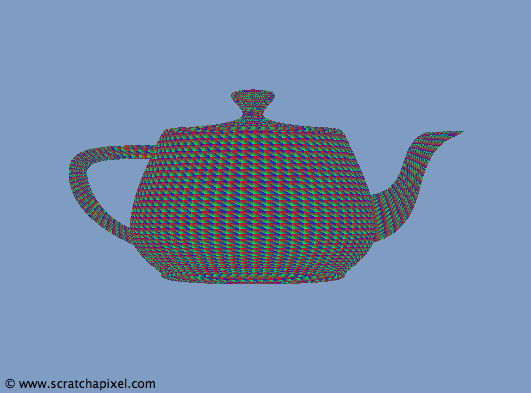
Creating the grid once we have this function is straightforward. We need to decide how many rows and vertices of quads we want, which defines the number of steps we take in u and v, compute the vertices' positions on the surface for these pairs of (u, v) values and connect these vertices to form the mesh (check the source code further down). The advantage of converting a Bézier surface into a polygon grid is that we can adapt the number of polygons (the resolution of the grid) based on some criteria, such as the curvature of the surface or its distance to the camera (a surface closer to the camera requires a higher definition. This is the principle of the REYES algorithm used by Pixar's renderer). What we render at the end is not the Bézier surface. Instead, we evaluate the Bézier surface as a polygon mesh which we can ray trace as a mesh (as we did with the polygon sphere in lesson 10).

Source Code

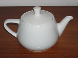
The renderer needs to access the teapot data, which we have saved in a separate file. The format is very similar to that of polygonal objects. We first have a series of vertices and 32 arrays of 16 integers, defining the position of the patches' control points in this array.

// Teapot data
const static uint16_t kTeapotNumPatches = 32; 
const static uint16_t kTeapotNumVertices = 306; 
uint32_t teapotPatches[kTeapotNumPatches][16] = { 
    {  1,   2,   3,   4,   5,   6,   7,   8,   9,  10,  11,  12,  13,  14,  15,  16}, 
    ... 
    {270, 270, 270, 270, 300, 305, 306, 279, 297, 303, 304, 275, 294, 301, 302, 271} 
}; 
 
float teapotVertices[kTeapotNumVertices][3] = { 
    { 1.4000,  0.0000,  2.4000}, 
    ... 
    { 1.4250, -0.7980,  0.0000} 
}; 

Finally, before the render starts, we need to convert each of these Bézier patches into a polygon grid. For each converted patch, we set the sixteen control points (lines 26-29), then construct a pair of (u, v) values for each vertex of the grid (we can control the resolution of the grid line 19), which is used to compute a position on the surface (line 33). The function returning this position computes the four auxiliary control points necessary to create a curve along the v direction using the u parameter. We can then use the v parameter to calculate the position on the surface along this curve. The rest of the code sets an array to connect the vertices (lines 36-45) and pushes the resulting polygon mesh to the list of objects (line 47).

Vec3f evalBezierCurve(const Vec3f *P, const float &t) 
{ 
    float b0 = (1 - t) * (1 - t) * (1 - t); 
    float b1 = 3 * t * (1 - t) * (1 - t); 
    float b2 = 3 * t * t * (1 - t); 
    float b3 = t * t * t; 
    return P[0] * b0 + P[1] * b1 + P[2] * b2 + P[3] * b3; 
} 
 
Vec3f evalBezierPatch(const Vec3f *controlPoints, const float &u, const float &v) 
{ 
    Vec3f uCurve[4]; 
    for (int i = 0; i < 4; ++i) uCurve[i] = evalBezierCurve(controlPoints + 4 * i, u); 
    return evalBezierCurve(uCurve, v); 
} 
 
void generatePolyTeapot(const Matrix44f &o2w, std::vector<Object *> &objects) 
{ 
    uint32_t divs = 16; 
    Vec3f *P = new Vec3f[(divs + 1) * (divs + 1)]; 
    uint32_t *nvertices = new uint32_t[divs * divs]; 
    uint32_t *vertices = new uint32_t[divs * divs * 4]; 
    Vec3f controlPoints[16]; 
    for (int np = 0; np < kTeapotNumPatches; ++np) { 
        // set the control points for the current patch                                                                                                                                                    
        for (uint32_t i = 0; i < 16; ++i) 
            controlPoints[i][0] = teapotVertices[teapotPatches[np][i] - 1][0], 
            controlPoints[i][1] = teapotVertices[teapotPatches[np][i] - 1][1], 
            controlPoints[i][2] = teapotVertices[teapotPatches[np][i] - 1][2]; 
        // generate grid                                                                                                                                                                                   
        for (uint16_t j = 0, k = 0; j <= divs; ++j) { 
            for (uint16_t i = 0; i <= divs; ++i, ++k) { 
                P[k] = evalBezierPatch(controlPoints, i / (float)divs, j / (float)divs); 
            } 
        } 
        // face connectivity
        for (uint16_t j = 0, k = 0; j < divs; ++j) { 
            for (uint16_t i = 0; i < divs; ++i, ++k) { 
                nvertices[k] = 4; 
                vertices[k * 4] = (divs + 1) * j + i; 
                vertices[k * 4 + 1] = (divs + 1) * (j + 1) + i; 
                vertices[k * 4 + 2] = (divs + 1) * (j + 1) + i + 1; 
                vertices[k * 4 + 3] = (divs + 1) * j + i + 1; 
            } 
        } 
 
        objects.push_back(new PolygonMesh(o2w, divs * divs, nvertices, vertices, P)); 
    } 
 
    delete [] P; 
    delete [] nvertices; 
    delete [] vertices; 
} 

The original teapot was much taller than the actual model. To get a render of the original teapot as designed by Newell, you need to scale it up by a factor of 4:3 along the y-axis. You also need to rotate the teapot along the z-axis by 90 degrees. In Newell's times, the z-axis and y-axis were swapped.

What's Next?

In the next chapter, we will learn about another technique called fast-forward differential to convert a Bézier patch into a grid. Nowadays, this technique is unnecessary: the conversion steps take a fraction of the overall time it takes to render the frame. However, it was valuable to speed up this pre-processing step when computers were slower.