Trilinear Interpolation
Reading time: 6 mins.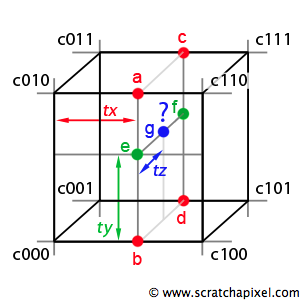
Trilinear interpolation is a direct extension of the bilinear interpolation technique. It can be seen as the linear interpolation of two bilinear interpolations: one for the front face of the cell and one for the back face. To compute e and f, we use two bilinear interpolations with the techniques described in the previous chapter. To compute g, we linearly interpolate e and f along the z-axis (using tz, which is the z coordinate of the sample point g).
Trilinear interpolation has the same strengths and weaknesses as its 2D counterpart. It's fast and easy to implement, but it doesn't produce very smooth results. However, for volume rendering or fluid simulation, where a very large number of lookups in 3D grids are performed, it is still a very good choice.
Here is a simple example of trilinear interpolation on a grid. Note that, like with bilinear interpolation, the results can be computed as a series of operations (lines 43 to 45) or as a sum of the 8 corners of cells weighted by some coefficients (lines 47 to 55).
template<typename T>
class Grid
{
public:
    unsigned nvoxels;  //number of voxels (cube)
    unsigned nx, ny, nz;  //number of vertices
    Vec3<T> *data;
    Grid(unsigned nv = 10) : nvoxels(nv), data(NULL)
    {
        nx = ny = nz = nvoxels + 1;
        data = new Vec3<t>[nx * ny * nz];
        for (int z = 0; z < nz + 1; ++z) {
            for (int y = 0; y < ny + 1; ++y) {
                for (int x = 0; x < nx + 1; ++x) {
                    data[IX(x, y, z)] = Vec3<t>(drand48(), drand48(), drand48());
                }
            }
        }
    }
    ~Grid() { if (data) delete [] data; }
    unsigned IX(unsigned x, unsigned y, unsigned z)
    {
        if (!(x < nx)) x -= 1; if (!(y < ny)) y -= 1; if (!(z < nz)) z -= 1;
        return x * nx * ny + y * nx + z;
    }
    Vec3<T> interpolate(const Vec3<T>& location)
    {
        T gx, gy, gz, tx, ty, tz;
        unsigned gxi, gyi, gzi;
        // remap point coordinates to grid coordinates
        gx = location.x * nvoxels; gxi = int(gx); tx = gx - gxi;
        gy = location.y * nvoxels; gyi = int(gy); ty = gy - gyi;
        gz = location.z * nvoxels; gzi = int(gz); tz = gz - gzi;
        const Vec3<T> & c000 = data[IX(gei, gyi, gzi)];
        const Vec3<T> & c100 = data[IX(gxi + 1, gyi, gzi)];
        const Vec3<T> & c010 = data[IX(gxi, gyi + 1, gzi)];
        const Vec3<T> & c110 = data[IX(gxi + 1, gyi + 1, gzi)];
        const Vec3<T> & c001 = data[IX(gxi, gyi, gzi + 1)];
        const Vec3<T> & c101 = data[IX(gxi + 1, gyi, gzi + 1)];
        const Vec3<T> & c011 = data[IX(gxi, gyi + 1, gzi + 1)];
        const Vec3<T> & c111 = data[IX(gxi + 1, gyi + 1, gzi + 1)];
#if 1
        Vec3<T> e = bilinear<Vec3<T> >(tx, ty, c000, c100, c010, c110);
        Vec3<T> f = bilinear<Vec3<T> >(tx, ty, c001, c101, c011, c111);
        return e * ( 1 - tz) + f * tz;
#else
        return
            (T(1) - tx) * (T(1) - ty) * (T(1) - tz) * c000 +
            tx * (T(1) - ty) * (T(1) - tz) * c100 +
            (T(1) - tx) * ty * (T(1) - tz) * c010 +
            tx * ty * (T(1) - tz) * c110 +
            (T(1) - tx) * (T(1) - ty) * tz * c001 +
            tx * (T(1) - ty) * tz * c101 +
            (T(1) - tx) * ty * tz * c011 +
            tx * ty * tz * c111;
#endif
    }
};

template<typename T>
void testTrilinearInterpolation()
{
    Grid<T> grid;
    for (unsigned i = 0; i < 1000; ++i) {
        // create a random location
        Vec3<T> result = grid.interpolate(Vec3<t>(drand48(), drand48(), drand48()));
    }
}
Implementation Details (2024 Update)
Since the lesson was first written, we have made some changes to the code (2024) to fix bugs. Checking the output of the code isn't as straightforward as it is with interpolation on 2D images. This is because 3D grids are mostly used to store and render volumetric objects, which requires a renderer that handles volumetrics to properly test the interpolation.
When the lesson was first written, the lesson on volume rendering wasn't available. This is no longer the case. We recommend checking the lesson on Volume Rendering to see a possible use case of 3D linear interpolation.
In the meantime, the code was improved to output a frame per slice in the output/upres grid. By looping through the output images, you can effectively see the result of the interpolation. Thanks to @kristopolous for this suggestion and making the changes to the code to support that idea.
Here is a visualization of the results that the program outputs. The initial 3D grid scr_grid3d has a resolution of 8x8x8, and the program aims to upres that grid to target_grid3d which is 128x128x128 in size. The program loops over every vertex of the upres grid (target_grid3d) and uses trilinear interpolation with data from the lower grid to set their own values. When you implement this technique, you need to be careful about a couple of things:
-
The number of vertices is the number of cells making up the dimension of the grid in any dimension plus 1 (in the code sample, the grid has equal dimensions in all three axes).
uint32_t grid_size = 8; // number of cells along the x, y and z-axis
uint32_t scale = 16;

uint32_t src_num_verts = grid_size + 1;
uint32_t target_num_verts = grid_size * scale + 1;
-
When making a lookup into the low-resolution grid, ensure that no index is greater than the lower grid size (hence the
std::min(grid_size, ...)when calculating the indices in the code).for (uint32_t z = 0; z < target_num_verts; ++z) { gz = float(z) / scale; gzi0 = uint32_t(gz); tz = gz - gzi0; gzi1 = std::min(grid_size, gzi0 + 1); // can't be greater than grid_size ...