Improved Perlin Noise
Reading time: 14 mins.A few years later (in fact, in 2002, so 17 years after Perlin published his first paper on noise), Perlin proposed a new, improved version of his noise function. The original noise function has two problems.
The smoothstep function is not ideal, and here is why...
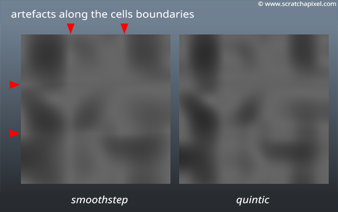
First, remember that the interpolant we used to interpolate the result of the dot product between the gradients and the vectors pointing toward the point within the cell is the smoothstep function. This function has the form \(3t^2 - 2t^3\). Remember that we used the derivative of this function (\(6t - 6t^2\)) to compute the Noise function partial derivatives. As explained in the previous chapter, these derivatives are useful to compute the "true" normal (true as in mathematically correct) of vertices displaced by a noise function. Now the problem with this is that the derivative of the smoothstep function derivative (what we call in mathematics the second order derivative or \(f''(x)\)) is not continuous when \(t=0\) or \(t=1\). The second-order derivative of the smoothstep function is \(6 - 12t\). So when \(t=0\) \(f''(x)=6\) and when \(t=1\), \(f''(x)=-6\). This is a problem because if the derivative of the function used to compute the normal of the displaced mesh is not continuous, then it will introduce a discontinuity in these normals wherever \(t=0\) and \(t=1\). That happens when the vertices of the displaced mesh are aligned with the edges of the noise grid cells (i.e., when the vertex's coordinates have integer values). These visual artifacts are visible in the image below (left).
It is essential to understand that while the analytical solution to compute the noise function derivative is correct mathematically; this doesn't mean that the result is necessarily visually what we look for. This is nothing more than a mathematical construct and may have properties we don't like. So while the results are mathematically correct, they create visual artifacts we would instead prefer to avoid.
Furthermore, most documents mentioning the problem of this function don't explain why we have this problem and provide a way of visualizing it. To better understand why the problem is there in the first place, you need to remember a detail about functions and function derivatives. In physics, a standard function is a function that allows you to compute the position of a moving object as a function of time. Let's call this function \(p(t)\). If you recall your lessons on physics, you can compute the speed of this object as the derivative of this function with respect to time, in other words, \(p'(t)=p(t)/\partial t\). And finally, you can compute the object acceleration as the derivative of the speed function with respect to time again or \(p''(t)=p'(t)/\partial t\). So, in essence you can see a function \(f(x)\) and its derivatives \(f'(x)\) and \(f''(x)\) as, respectively the position, the speed, and the acceleration of an object. In our example, the smoothstep function is, by analogy, the position, the first-order derivative of the smoothstep function that we used to compute the tangent is the speed, and finally the second-order derivative of the smoothstep function is the acceleration. Of course, these are just analogies. But the point is, if the acceleration has discontinuities, then we can expect the speed to change abruptly from time to time. In our particular case, if the smoothstep function second order derivative has discontinuities, then we can expect the tangent to vary abruptly from time to time. And that's precisely what causes the visual artifacts at the cell boundaries. The normals in these regions change suddenly.
In computer graphics and mathematics, when the original function is continuous, we speak of geometry continuity, and we say the function is C0 (or G0 when we deal with geometry). If the function derivative is continuous, we speak of tangent continuity (C1 or G1). And when the function second order derivative is also continuous, we speak of curvature continuity; in other word, the curvature where two curves or two surfaces join is the same for the curves or two surfaces at the point of contact).
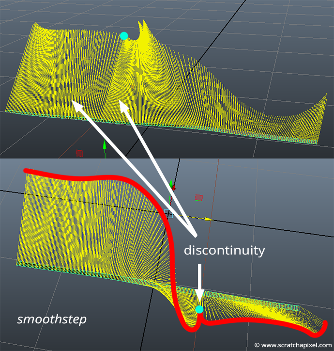
The image below shows a slice of the noise function and its analytically computed normals. It is clear that the orientation of the normals and the direction of these are not the same on each side of the cell boundary.
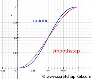
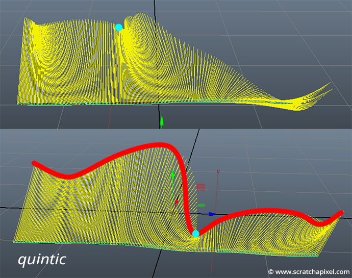
Hopefully, there is a solution. Well, if the only problem is that the second-order derivative of the smoothstep function is discontinuous, then all we need to do to fix the problem is to choose a function for the interpolant with a second-order derivative, obviously, continuous. There are quite a few of them that have a similar shape to the smoothstep function, but Perlin choose this quintic function (figure 1):
$$6t^5-15t^4+10t^3.$$Its first-order derivative is:
$$30t^4-60t^3+30t^2.$$And its second-order derivative is:
$$120t^3-180t^2+60t.$$As you can see, this function is continuous (when t=0 and t=1, the function is equal to 0).
Choosing random gradients is not ideal, and here is why...
The next problem is that because the gradients are chosen randomly, sometimes the gradient directions are aligned along the same axis or along the cell's diagonal, as shown in figure 2 [missing]. The noise function tends to take on very high values in these regions (close to 1), causing the "splotchy appearance" of the original Noise implementation in parts.
Hopefully, this problem can be solved easily by replacing the 256 random directions with a set of 12 directions that are different from each other (excluding situations in which these gradients would point along the same direction). The permutation table provides plenty of randomnesses, so it doesn't matter if these 12 vectors are predefined. Perlin, in his 2002 paper, decided to choose the following vectors:
$$ \begin{array}{l} (1,1,0),(-1,1,0),(1,-1,0),(-1,-1,0),\\ (1,0,1),(-1,0,1),(1,0,-1),(-1,0,-1),\\ (0,1,1),(0,-1,1),(0,1,-1),(0,-1,-1) \end{array} $$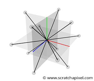
Though keep in mind that our permutation table returns integers in the range [0,255], so to choose one of these vectors randomly, we would need to do something like P[Hash(x,y,z)] % 12. We don't like to use the modulo operator too much because it's slower than bitwise operators. It requires handling negative values differently than positive ones (bitwise operators fix this problem). To replace the modulo operator with a bitwise operator, Perlin proposes to extend the array of 12 vectors to 16 vectors, adding to the first 12 the following 4 directions:
$$ \begin{array}{l} (1,1,0),(-1,1,0),(0,-1,1), (0,-1,-1). \end{array} $$We already used these directions, but Perlin claims that because the first 12 directions form a regular tetrahedron, adding some of these directions redundantly doesn't introduce any bias in the texture.
The final result has the same non-directional appearance as the original distribution but less clumping.
The splotchy-like appearance is no longer visible (check out the comparison image below). Implementing this change is quite simple. Our hash function returns numbers in the range [0,255], so we need to use another bitwise operator to set this number to the range [0,15].
uint8_t p = hash(xi, yi, zi) & 15;
Then note that because all directions are defined with 0 and 1, the dot product is simplified into a sum of the coordinates of the right-hand vector.
// float a = dot(c000, p000);
// float a = c000.x * p000.x + c000.y * p000.y + c000.z * p000.z;
// for the gradient (1, 1, 0), for instance, this simplifies to:
float a = 1 * p000.x + 1 * p000.y + 0 * p000.z = p000.x + p000.y;
We can move this code into its function:
float gradientDotV(
    // a value between 0 and 255
    uint8_t perm,
    // vector from one of the corners of the cell to the point where the noise function is computed
    float x, float y, float z)
{
    switch(perm & 15) {
        case  0: return  x + y;  //(1,1,0)
        case  1: return -x + y;  //(-1,1,0)
        case  2: return  x - y;  //(1,-1,0)
        case  3: return -x - y;  //(-1,-1,0)
        case  4: return  x + z;  //(1,0,1)
        case  5: return -x + z;  //(-1,0,1)
        case  6: return  x - z;  //(1,0,-1)
        case  7: return -x - z;  //(-1,0,-1)
        case  8: return  y + z;  //(0,1,1),
        case  9: return -y + z;  //(0,-1,1),
        case 10: return  y - z;  //(0,1,-1),
        case 11: return -y - z;  //(0,-1,-1)
        case 12: return  y + x;  //(1,1,0)
        case 13: return -x + y;  //(-1,1,0)
        case 14: return -y + z;  //(0,-1,1)
        case 15: return -y - z;  //(0,-1,-1)
    }
}

float eval(...)
{
    ...
    float a = gradientDotV(hash(xi0, yi0, zi0), x0, y0, z0);
    float b = gradientDotV(hash(xi1, yi0, zi0), x1, y0, z0);
    float c = gradientDotV(hash(xi0, yi1, zi0), x0, y1, z0);
    float d = gradientDotV(hash(xi1, yi1, zi0), x1, y1, z0);
    float e = gradientDotV(hash(xi0, yi0, zi1), x0, y0, z1);
    float f = gradientDotV(hash(xi1, yi0, zi1), x1, y0, z1);
    float g = gradientDotV(hash(xi0, yi1, zi1), x0, y1, z1);
    float h = gradientDotV(hash(xi1, yi1, zi1), x1, y1, z1);
    ...
}
The image below shows a comparison between the original Perlin noise implementation (left) and the improved version (right):
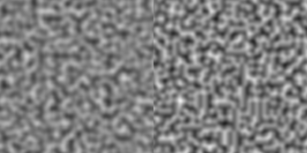
While not significantly different, the two implementations give different results. The improved version creates vertical and horizontal lines you don't see in the original version. This is because, in the enhanced version, the gradients are aligned along the xy, xz, and yz planes. While choosing a quintic function as an interpolant definitely reduces the visual artifacts and can be called an improvement, using predefined gradients over random gradients is not necessarily good. You can find the complete implementation of the improved version in the last chapter of this lesson.
inline
float quintic(const float &t)
{
    return t * t * t * (t * (t * 6 - 15) + 10);
}

inline
float quinticDeriv(const float &t)
{
    return 30 * t * t * (t * (t - 2) + 1);
}

class PerlinNoise
{
    ...
    /* inline */
    uint8_t hash(const int &x, const int &y, const int &z) const
    { return permutationTable[permutationTable[permutationTable[x] + y] + z]; }

    float gradientDotV(
        // a value between 0 and 255
        uint8_t perm,
        // vector from one of the corners of the cell to the point where the noise function is computed
        float x, float y, float z) const
    {
        switch (perm & 15) {
            case  0: return  x + y;  //(1,1,0)
            case  1: return -x + y;  //(-1,1,0)
            case  2: return  x - y;  //(1,-1,0)
            case  3: return -x - y;  //(-1,-1,0)
            case  4: return  x + z;  //(1,0,1)
            case  5: return -x + z;  //(-1,0,1)
            case  6: return  x - z;  //(1,0,-1)
            case  7: return -x - z;  //(-1,0,-1)
            case  8: return  y + z;  //(0,1,1),
            case  9: return -y + z;  //(0,-1,1),
            case 10: return  y - z;  //(0,1,-1),
            case 11: return -y - z;  //(0,-1,-1)
            case 12: return  y + x;  //(1,1,0)
            case 13: return -x + y;  //(-1,1,0)
            case 14: return -y + z;  //(0,-1,1)
            case 15: return -y - z;  //(0,-1,-1)
        }
    }

    float eval(const Vec3f &p, Vec3f& derivs) const
    {
        int xi0 = ((int)std::floor(p.x)) & tableSizeMask;
        int yi0 = ((int)std::floor(p.y)) & tableSizeMask;
        int zi0 = ((int)std::floor(p.z)) & tableSizeMask;

        int xi1 = (xi0 + 1) & tableSizeMask;
        int yi1 = (yi0 + 1) & tableSizeMask;
        int zi1 = (zi0 + 1) & tableSizeMask;

        float tx = p.x - ((int)std::floor(p.x));
        float ty = p.y - ((int)std::floor(p.y));
        float tz = p.z - ((int)std::floor(p.z));

        float u = quintic(tx);
        float v = quintic(ty);
        float w = quintic(tz);

        // generate vectors going from the grid points to p
        float x0 = tx, x1 = tx - 1;
        float y0 = ty, y1 = ty - 1;
        float z0 = tz, z1 = tz - 1;

        float a = gradientDotV(hash(xi0, yi0, zi0), x0, y0, z0);
        float b = gradientDotV(hash(xi1, yi0, zi0), x1, y0, z0);
        float c = gradientDotV(hash(xi0, yi1, zi0), x0, y1, z0);
        float d = gradientDotV(hash(xi1, yi1, zi0), x1, y1, z0);
        float e = gradientDotV(hash(xi0, yi0, zi1), x0, y0, z1);
        float f = gradientDotV(hash(xi1, yi0, zi1), x1, y0, z1);
        float g = gradientDotV(hash(xi0, yi1, zi1), x0, y1, z1);
        float h = gradientDotV(hash(xi1, yi1, zi1), x1, y1, z1);

        float du = quinticDeriv(tx);
        float dv = quinticDeriv(ty);
        float dw = quinticDeriv(tz);

        float k0 = a;
        float k1 = (b - a);
        float k2 = (c - a);
        float k3 = (e - a);
        float k4 = (a + d - b - c);
        float k5 = (a + f - b - e);
        float k6 = (a + g - c - e);
        float k7 = (b + c + e + h - a - d - f - g);

        derivs.x = du *(k1 + k4 * v + k5 * w + k7 * v * w);
        derivs.y = dv *(k2 + k4 * u + k6 * w + k7 * v * w);
        derivs.z = dw *(k3 + k5 * u + k6 * v + k7 * v * w);

        return k0 + k1 * u + k2 * v + k3 * w + k4 * u * v + k5 * u * w + k6 * v * w + k7 * u * v * w;
    }
    ...
};
What's Next?
This concludes our lesson on Perlin noise. The lesson is extensive already, but there is undoubtedly a lot more to say about noise functions. First, quite a few more ways of generating procedural noise exist. Some other standard methods are the wavelet noise (developed by Pixar), the Gabor noise, and the simplex noise, which is also a kind of noise created by Ken Perlin. We will write lessons on each one of these techniques in the future.
Finally, judging the quality of noise implementation against others is essential. How do we do that? We already mentioned the qualities that a noise function should have although. Among these qualities, the noise should have a distribution of frequencies as uniform as possible and yet still appear random and smooth. One way to determine whether a given noise function fits this criterion is to analyze its output in the frequency domain. We will also learn about this technique in future lessons.
How to Use the Noise Function?
A procedural noise function, in general, can be used for many things:
-
Terrain: in this lesson, we just studied the implementation of the function itself, though we also showed how to use it to create something like a terrain. We haven't shown yet how to create terrains with really intricate and realistic surface details using the noise function. We will show this technique in a separate lesson yet to be published.
-
Water surfaces can also be used to simulate a water surface. By offsetting the y coordinative of the input point, it is possible to animate the displaced surface like waves. This simple technique works well though there are better methods to simulate water surfaces.
-
Procedural noise can also be used to add surface details to volumes such as cloud. We use the noise function in the lesson on volume rendering to simulate the appearance of various cloudy shapes.
-
Texturing: finally, it can be used, of course, to add texture details to surfaces. It can be used to modulate any input of the shader, such as the color, the specular, or add some bump to the surface of an object.
-
Animation: the noise function can also add some noise to animations. A typical use case, for example, is to add some noise to a camera animation to simulate some camera shakes.
References
Improving Noise. Ken Perlin (2002)
State of the Art in Procedural Noise Functions. A. Lagae and al. (2010)