Using Perlin Noise to Create a Terrain Mesh
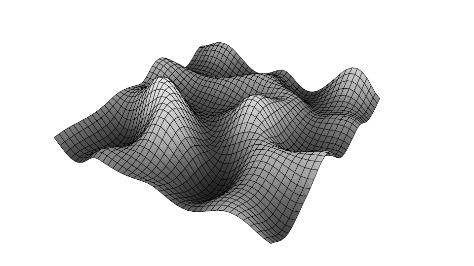
Reading time: 7 mins.In this chapter, we will learn about a fun technique that uses a 2D Perlin noise to displace the vertices of a mesh to create a terrain. As we mentioned in the first lesson on noise, the noise function is a key "procedural texture" primitive from which more complex procedural textures can be created, such as the fractal or the turbulence pattern. We will show an example of a terrain generated using a simple noise function first (image below) and a fractal pattern next.
This technique will help us understand better the importance of computing the Perlin noise function's derivatives, which is the next chapter's topic.
XX TODO. We are missing an image here that shows the mapping between the image and the mesh XX
The idea behind this technique is straightforward and similar to what we call displacement mapping. If you look at the grid from the top, you can see that if you overlay the noise image onto the grid, you get a perfect match: each grid vertex corresponds to a pixel in the noise image. As you know, we can define the coordinates of the pixels in some normalized device coordinates (the pixel coordinates are then in the range from [0,1]). The same can be done with the grid vertices: these are technically called texture coordinates. Let's look at the code we shall use to create the grid:
PolyMesh* createPolyMeshPlane(
    uint32_t width = 1,
    uint32_t height = 1,
    uint32_t subdivisionWidth = 40,
    uint32_t subdivisionHeight = 40)
{
    PolyMesh *poly = new PolyMesh;
    poly->numVertices = (subdivision with + 1) * (subdivisionHeight + 1);
    poly->vertices = new Vec3f[poly->numVertices];
    poly->st = new Vec2f[poly->numVertices];
    float invSubdivisionWidth = 1.f / subdivisionWidth;
    float invSubdivisionHeight = 1.f / subdivisionHeight;
    for (uint32_t j = 0; j <= subdivisionHeight; ++j) {
        for (uint32_t i = 0; i <= subdivisionWidth; ++i) {
            poly->vertices[j * (subdivisionWidth + 1) + i] = Vec3f(width * (i * invSubdivisionWidth - 0.5), 0, height * (j * invSubdivisionHeight - 0.5));
            poly->st[j * (subdivisionWidth + 1) + i] = Vec2f(i * invSubdivisionWidth, j * invSubdivisionHeight);
        }
    }

    poly->numFaces = subdivisionWidth * subdivisionHeight;
    poly->faceArray = new uint32_t[poly->numFaces];
    for (uint32_t i = 0; i < poly->numFaces; ++i)
        poly->faceArray[i] = 4;

    poly->verticesArray = new uint32_t[4 * poly->numFaces];
    for (uint32_t j = 0, k = 0; j < subdivisionHeight; ++j) {
        for (uint32_t i = 0; i < subdivisionWidth; ++i) {
            poly->verticesArray[k] = j * (subdivisionWidth + 1) + i;
            poly->verticesArray[k + 1] = j * (subdivisionWidth + 1) + i + 1;
            poly->verticesArray[k + 2] = (j + 1) * (subdivisionWidth + 1) + i + 1;
            poly->verticesArray[k + 3] = (j + 1) * (subdivisionWidth + 1) + i;
            k += 4;
        }
    }

    return poly;
}
The texture coordinates of the vertex are computed in line 16. This is also a space where the coordinates are in the range from [0,1]. The vertex in the upper left corner of the grid has the texture coordinates [0,0], while the vertex in the lower-right coordinate has the texture coordinate [1,1]. Thus, it becomes easy to use the vertex texture coordinates to look up the noise image.
In this example, we baked the values from the 2D noise function in an image and read the noise values from that image (we showed how to do that in the previous chapter). In practice, we would more likely evaluate the 2D noise function. When an image is used to displace the vertices of an object, we say that this image is a height map (or displacement map).
In the case of a height map, we generally use the brightness (the luminance, for example) of the pixels' color to control the displacement amplitude. Typically, the brighter the pixel, the greater the displacement, though, of course, you can map the pixel value to displacement in a completely different way if you wish. It all depends on the effect you intend to create. All you need to remember is that you use an image to somehow control the amount by which the object's vertices are displaced or moved along the normal (the direction perpendicular to the mesh surface. In the case of a plane laying in the xz-plane, the mesh normal is simply (0,1,0) everywhere).
for (unsigned j = 0; j < imageHeight; ++j) {
    for (unsigned i = 0; i < imageWidth; ++i) {
        // Perlin noise is in the range [-1:1]
        float perlinNoise = PerlinNoise::evalAtPoint(Vec3f(i, j, 0) * (1 / 128.f));
        noiseMap[j * imageWidth + i] = (perlinNoise + 1) * 0.5;
    }
}

// displace
for (uint32_t i = 0; i < poly->numVertices; ++i) {
    Vec2f st = poly->st[i];
    uint32_t x = std::min(static_cast<uint32_t>(st.x * imageWidth), imageWidth - 1);
    uint32_t y = std::min(static_cast<uint32_t>(st.y * imageHeight), imageHeight - 1);
    poly->vertices[i].y = 2 * noiseMap[y * imageWidth + x] - 1;
}
Keep in mind that the values of the Perlin noise are in the range from [-1,1]. But we remapped these values to the range [0,1] when we stored the values in the image buffer (line 5). However, the values are mapped again back in the range from [-1,1] when we displace the vertices later on (line 15) because that way, the mesh will stay centered around the origin along the y-axis. We will push the vertices upward (if the values are greater than 0) or downward (if the values are lower than 0), and if the value is 0, the vertex y-coordinate will stay 0.
If you render this mesh with the noise image applied on top as a texture, you should get something similar to the first image of this chapter. Note how the white/bright area of the noise image corresponds to bumps in the mesh, while dark regions of the image correspond to dents or valleys (and note how the displacement is proportional to the pixel values).
As mentioned in the introduction of this chapter, you can use more interesting procedural patterns to displace the mesh vertices, such as a fractal pattern which can be constructed as a weighted sum of noise layers. Check the previous lesson on noise to learn how to generate a fractal pattern using the noise function as a building block. Here is the code to generate the fractal image that was used to displace the mesh:
uint32_t numLayers = 5;
float maxVal = 0;
for (uint32_t j = 0; j < imageHeight; ++j) {
    for (uint32_t i = 0; i < imageWidth; ++i) {
        float fractal = 0;
        float amplitude = 1;
        Vec3f pt = Vec3f(i, j, 0) * (1 / 128.f);
        for (uint32_t k = 0; k < numLayers; ++k) {
            fractal += (1 + PerlinNoise::evalAtPoint(pt)) * 0.5 * amplitude;
            pt *= 2;
            amplitude *= 0.5;
        }
        if (fractal > maxVal) maxVal = fractal;
        noiseMap[j * imageWidth + i] = fractal;
    }
}

for (uint32_t i = 0; i < imageWidth * imageHeight; ++i)
    noiseMap[i] /= maxVal;
A fractal image generally contains higher frequency details than a single layer of noise. Thus, to see these details in the displacement, you will likely have to increase the density of the mesh itself. Here is a render of the mesh displaced with a fractal image.
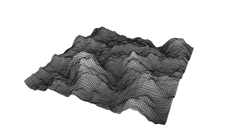
As suggested in the previous lesson, this technique can generate realistic terrains (hopefully, the image above is convincing enough). We can also use the noise function to create and animate water surfaces. In this example, the procedural pattern we used (a fractal) is pretty simple. You can play with the parameters a bit to modify the look of the terrain, but to increase the realism of the terrain, we would need to add effects such as erosion. But we will leave that topic for another lesson.
As a final note, we haven't computed the normal of the mesh after displacement. How do we do that? This is the topic of our next chapter. We will learn how to compute a "true" normal at the vertex position after displacement using the noise function derivatives.