Introduction
Reading time: 17 mins.To the physicist, unpredictable changes of any quantity V varying in time t are known as noise. (The Science of Fractal Images, Richard F. Voss).
This lesson explains the concept of noise in a very simple (almost naive) form. You will learn what noise is, its properties, and what you can do with it. Noise is not a complicated concept, but it has many subtleties. Using it right requires an understanding of how it works and how it is made. To create some images and experiment with various parameters, we will implement a simple (but fully functional) version of a noise function known as value noise. Keep in mind while reading this lesson that we will be overlooking many techniques that are too complex to study here thoroughly. This is just a brief introduction to noise and a few of its possible applications. The website offers many lessons where each topic mentioned in this lesson can be studied individually (aliasing, texture generation, complex noise functions, landscape cloud, and water surface generation) and a few advanced programming techniques such as bitwise arithmetic, hashing, etc.).
Historical Background
Noise was developed in the mid-'80s as an alternative to using images for texturing objects. We can map objects with images to add visual complexity to their appearance. In CG, this is known as texture mapping. However, in the mid-'80s, computers had minimal memory, and images used for texturing would not easily fit in RAM. People working in CG studios started to look for alternative solutions. Objects that were rendered with solid colors seemed too clean. They needed something to break this clean look by modulating objects' visual properties (color, shininess) across their surface. In programming, we usually use random number generators whenever we need to create random numbers. However, using an RNG (random number generator) to add variation to the appearance of a 3D object isn't sufficient. Random patterns we can observe in nature are usually smooth. Two points on the surface of a real object typically look the same when they are close to each other. But two points on the surface of the same object far apart can look very different. In other words, local changes are gradual, while global changes can be large. An RNG does not have this property. Every time we call them, they return numbers unrelated (uncorrelated) to each other. Therefore calling this function is likely to produce two very different numbers. This would be unsuitable for introducing a slight variation to the visual appearance of two spatially close points. Here is an example: let's observe the image of a natural rock (Figure 1 left), and let's assume that our task is to create a CG image that reproduces the look of this object. You can't use textures (the most obvious solution is to take this image and map it on a plane). We have a plane that, without texturing, looks completely flat (uniform color). This example is interesting because we can observe that the rock pattern is made of three primary colors: green, pink, and grey. These colors are distributed in equal amounts across the surface of the rock. The first obvious solution to this problem is to open this image with Photoshop, for instance, pick up each of these three average colors to reuse them in a program that procedurally generates a pattern more or less similar to our reference picture. This is what the following code does. However, for now, all we can do to create a variation from pixel to pixel is to use the C drand48() function, which returns a random value in the range [0:1].
void GenerateRandPattern()
{
    unsigned imageWidth, imageHeight;
    imageWidth = imageHeight = 512;
    static const unsigned kNumColors = 3;
    Color3f rockColors[ kNumColors ] = {
        { 0.4078, 0.4078, 0.3764 },
        { 0.7606, 0.6274, 0.6313 },
        { 0.8980, 0.9372, 0.9725 } };
    std::ofstream ofs( "./rockpattern.ppm" );
    ofs << "P6\n" << imageWidth << " " << imageHeight << "\n255\n";
    for ( int j = 0; j < imageWidth; ++j )
    {
        for ( int i = 0; i < imageHeight; ++i )
        {
            unsigned colorIndex = std::min( unsigned( drand48 () * kNumColors ), kNumColors - 1 );
            ofs << uchar( rockColors[ colorIndex ][ 0 ] * 255 ) <<
                   uchar( rockColors[ colorIndex ][ 1 ] * 255 ) <<
                   uchar( rockColors[ colorIndex ][ 2 ] * 255 );
        }
    }
    ofs.close();
}
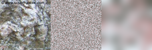
As you can see in the middle of figure 1, the result of this program is not convincing (in fact, this pattern has a name; it is called white noise. We will explain what white noise is later, but for now remember that it looks like the image in the middle of Figure 1). We use an RNG to select a color for each pixel of the procedurally generated texture, which causes a large variation from pixel to pixel. To improve the result, we copied a small region of the texture (10x10 pixels) which we resized (enlarged) to the dimension of the original image (256x256 pixels). Enlarging this portion of the frame will blur the pixels, but to make the result even smoother, we applied a gaussian blur on top in Photoshop. We haven't yet matched the reference image well, but as you can see, the resulting image (right image in Figure 1) is already better than the original one (middle). Locally, we have small variations (small changes in color from pixel to color), while globally, we have larger variations (a mix of the three input colors).
The conclusion of this experiment is that to create a smooth random pattern, we need to assign random values at a fixed position on a grid which we call a lattice (in our example, the grid corresponds to the pixel locations of our 10x10 input image) using an RNG, and blur these values using something equivalent to a gaussian blur (a smoothing function to blur these random values). The next chapter will show you how this can be implemented. But for now, all you need to remember is that noise (within the context of computer graphics) is a function that blurs random values generated on a grid (which we often refer to as a lattice).
The process we just described is similar to bilinear interpolation (see the lesson on interpolation). In the following example (Figure 2), we created a 2D grid of size 10x10, set a random number at each vertex of the grid, and used linear interpolation to render a larger image.
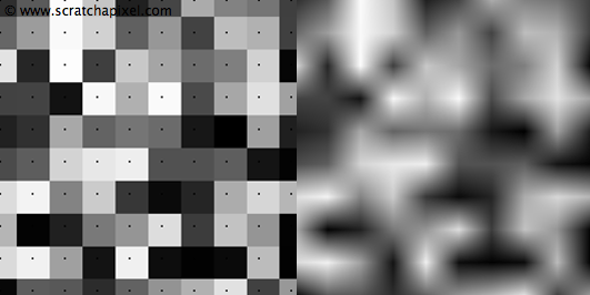
As you can see, the quality of the result is not very good. We have pointed out in the lesson on interpolation that bilinear interpolation was the most straightforward possible technique for interpolating data and that to improve the quality of the result (if needed), it was possible to use interpolants (the function used to interpolate the data) of higher degrees. In the next chapter, we will write a noise function that provides better results than this simple linear interpolation of 2D grid data.
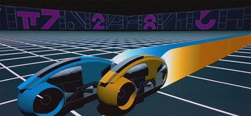
Ken Perlin wrote the most popular implementation of noise in 1983 (and is probably the first one of its kind) while working on the 1982 version of the film Tron (© Walt Disney Pictures). If you go on his website (or search for Ken Perlin in your favorite search engine), you will easily find a reference to the page where Ken Perlin himself gives the history of his noise pattern. Ken Perlin was awarded an Academy Award for Technical Achievement from the Academy of Motion Picture Arts and Sciences for his contribution to the film in 1997. He presented his work at Siggraph in 1984 and published a paper in 1985, "An Image Synthesiser," which is seminal in texture synthesis. It is highly recommended that you read this paper if you are interested in learning about the basics of the noise function (and its development history). Perlin noise is explained in the lesson Noise Part 2.
The World of Procedural Texturing
The development of noise leads to a new area of research in computer graphics. Noise can be seen as a basic building block from which many interesting procedural textures (also called solid textures, see the lesson on Texturing) can be generated. In the world of procedural texturing, many types of textures can be generated which are not always trying to resemble natural patterns. Writing a program for generating a brick wall type of pattern is simple. Some patterns can be regular, irregular, or stochastic (non-deterministic).
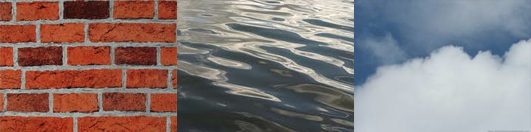
Apart from regular patterns (which only obey geometric rules and are perfect in shape), all other patterns can use noise to introduce irregularities or drive the apparent randomness to the procedurally generated texture. After Ken Perlin introduced his version of the noise function, many people in the CG community started to use it for modeling complex materials and objects, such as terrains, clouds, or animating water surfaces. Noise is not limited to changing the visual appearance of an object. Still, it can also be used for procedural modeling, to displace the surface of an object (for generating terrains), or control the density of a volume (cloud modeling). By offsetting the noise input from frame to frame, we can also use it for procedurally animating objects. It was the favorite method until the mid-'90s for animating water surfaces (Jerry Tessendorf proposed a more practical approach in the late 90s. See the lesson on Animating Ocean Waves).
Some examples of simple solid textures (fractals) are given in the last chapter of this lesson. The lesson on Texture Synthesis will provide you with more information on this topic.
Main Advantage/Disadvantage of Noise
As we mentioned in the introduction, noise has the advantage of being compact. It doesn't use a lot of memory compared to texture mapping, and implementing a noise function is not very complex (a noise function requires little data storage). From this very basic function, it is also possible to create a large variety of textures (we will give some examples in the last chapter of this lesson). Finally, using noise to add texture to an object doesn't require any parametrization of the surface, which is usually needed for texture mapping (where we need texture coordinates).
On the other hand, they are usually slower than texture mapping. The noise function requires the execution of quite a few math operations (even if they are simple, there are quite a few), while texture mapping only requires access to the pixels of a texture (an image file) loaded in memory.
Properties of an Ideal Noise
If it is possible to list all the properties that an ideal noise should have, not every implementation of the noise function matches them all (and quite a few versions exist).
Noise is pseudo-random, and this is probably its main property. It looks random but is deterministic. Given the same input, it always returns the same value. If you render an image for a film several times, you want the noise pattern to be consistent/predictable. Or if you apply this noise pattern to a plane, for example, you want that pattern to stay the same from frame to frame (even if the camera moves or the plane is transformed. The pattern sticks to the plane. We say that the function is invariant: it doesn't change under transformations).
The noise function always returns a float, no matter the dimension of the input value. The dimension of the point is given to the name of the noise. A 1D, 2D, and 3D noise functions take 1D, 2D and 3D points as input parameters. There is even a 4D noise that takes a 3D point as an input parameter, and an additional float value is used to animate the noise pattern over time (time-varying solid texture). Examples of 1D and 2D noise are given in this lesson. 3D and 4D noise examples are shown in the lesson Noise Part 2. In mathematical terms, we say that the noise function is a mapping from Rn to R (where n is the dimension of the value passed to the noise function). It takes an n-dimensional point with real coordinates as input and returns a float. 1D noise is used for animating objects, and 2D and 3D noise is used for texturing objects. 3D noise helps modulate the density of volumes.
Noise is band limited. Remember that noise is mainly a function, which you can see as a signal (if you plot the function, you get a curve which is your signal). In signal processing, it's possible to convert a signal from the spatial domain to the frequency domain. This operation gives a result from which it is possible to see the different frequencies of a signal. Don't worry too much if you don't understand what it means to go from spatial to frequency space (it is off-topic here, but you can check the lesson on Fourier Transform). All you need to remember is that the noise function is potentially made of multiple frequencies (low frequencies account for large-scale changes, and high frequencies account for small-scale changes). But one of these frequencies dominates all the others. And this one frequency defines both the visual and frequency (if you look at your signal in frequency space) appearance/characteristic of your noise function. Why should we care about the frequency of a noise function? When the noise is small in the frame (imaging an object textured with noise far away from the camera), it becomes white noise again, which is a cause of what we call, in our jargon, aliasing. This is illustrated in Figure 4.
In the background of this image, neighbor pixels take random values. Not only is this not visually pleasant and realistic, but if you render a sequence of images, the values of the pixels in this area will change drastically from frame to frame (Figure 4). Aliasing is related to the topic of sampling, which is a very large and critical topic in computer graphics. We invite you to read the lesson on sampling if you want to understand what's causing this unwanted effect.
We mentioned that noise uses a smooth function to blur random values generated at lattice points. Functions in mathematics have properties. Two of them are of particular interest in the context of this lesson: continuity and differentiability. Explaining what these are is off-topic here, but with a simple example, you will intuitively understand what they mean. A derivative is a line tangent to a curve profile, as shown in Figure 5. However, if the function is not continuous, computing this derivative is impossible (a function can also be continuous but not differentiable everywhere, as shown in Figure 5 on the right). For reasons we will explain later, computing derivatives of the noise function will be needed in some places, and it is best to choose a smooth, continuous, and differentiable function. The original implementation of the noise function by Ken Perlin used a function that wasn't continuous, and he suggested another one a few years later to correct this problem.
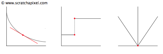
We can find out the tangent anywhere on the noise curve. If there's a place on this curve where this tangent can't be found or where it changes abruptly, it causes what we call discontinuities.
Finally, when you look at the noise applied to an object, ideally, you shouldn't see the repetition of the noise pattern. As we started to suggest, noise can only be computed from a grid of a predefined size. In the example above, we chose a 10x10 grid. What would we do if we were to calculate noise outside the boundaries of that grid? Noise is like a tile; to cover a larger area with tiles of a particular dimension, you need to lay many of these tiles next to each other. But there would be two obvious problems with this approach. At the boundaries of the tile, the noise pattern would be discontinuous.
// Figure 6 insert figure side by side many noise tiles repetition then periodic but repetition.

Ideally, you want an invisible transition from tile to tile to cover an infinitely large area without ever seeing a seam. When a 2D texture is seamless in CG, it is said to be periodic in both directions (x and y). The word tileable is also sometimes used but is confusing. Any texture is tileable. But it might not be seamless. Your noise function should be designed so that the pattern is periodic. Furthermore, because you have used many tiles with the same pattern, you might spot the repetition of that pattern. The solution to this problem is harder to explain at this stage of the lesson. What you need to know for now is that the pattern created by the noise function has no large features (all the features have roughly the same size, remember what we said about the function being band limited). If you zoom out, you will not see the repetition of large features because they are not in the function. As for the other smaller features that the noise is made of, they are too small to be seen by the time you have zoomed out quite a lot. The trick (because it is one) for making the pattern invisible is to make it large enough (make the grid of lattice points large enough) so that by the time you have covered your entire screen, the features are too small in frame to be seen. We will demonstrate this effect in the next chapter.