Rasterization

Rasterization: a Practical Implementation

Improving the Rasterization Algorithm

Aliasing and Anti-Aliasing

The techniques presented in previous chapters lay the foundation of the rasterization algorithm. However, we have implemented these techniques in a very basic manner. The GPU rendering pipeline and other rasterization-based production renderers employ the same concepts but use highly optimized versions of these algorithms. Detailing all the different tricks used to speed up the algorithm goes well beyond the scope of an introduction. We will quickly review some of them now but plan to devote a lesson to this topic in the future.

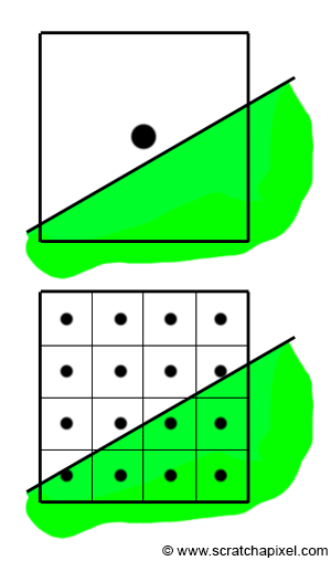
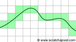
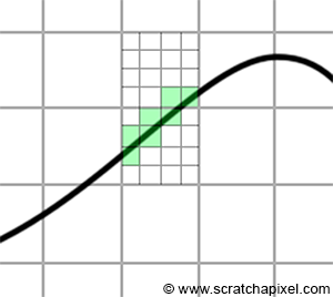
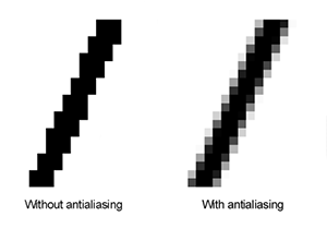
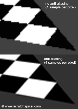
First, let's consider a fundamental problem with 3D rendering. If you zoom in on the image of the triangle we rendered in the previous chapter, you will notice that the edges of the triangle are irregular (this irregularity is not specific to the edge of the triangle; you can also observe that the checkerboard pattern is uneven on the edges of the squares). The steps easily visible in figure 1 are called jaggies. These jagged or stair-stepped edges (whichever term you prefer) are not an artifact. They are simply the result of breaking down the triangle into pixels. With rasterization, we break down a continuous surface (the triangle) into discrete elements (pixels), a process already mentioned in the Introduction to Rendering. The challenge is akin to attempting to represent a continuous curve or surface with Lego bricks. It's just not possible without noticing the bricks (figure 2). The solution in rendering is called anti-aliasing (AA). Rather than rendering only one sample per pixel, we divide the pixel into sub-pixels and perform the coverage test for each. Of course, each sub-pixel is merely another "brick," and this doesn't entirely solve the problem. Nonetheless, it allows for capturing the edges of objects with slightly more precision. Pixels are typically divided into an N by N grid of sub-pixels, where N is usually a power of 2 (2, 4, 8, etc.), though it technically can be any value greater than or equal to 1 (1, 2, 3, 4, 5, etc.). There are various methods to address this aliasing issue, and the described technique falls under sampling-based anti-aliasing methods.

The final pixel color is computed as the sum of all sub-pixel colors divided by the total number of sub-pixels. For example, imagine the triangle is white. If only 2 or 4 samples overlap the triangle, the final pixel color will be equal to (0+0+1+1)/4=0.5. The pixel will not be completely white, but neither will it be completely black. Instead of a "binary" transition between the edge of the triangle and the background, the transition is more gradual, mitigating the stair-stepped pixel artifact. This technique is known as anti-aliasing. To fully understand anti-aliasing, one needs to delve into signal processing theory, which is a vast and complex topic.

Choosing N as a power of 2 is beneficial because most processors today can execute several instructions in parallel, and the number of parallel instructions is also generally a power of 2. You can find information on the Web about things like SSE instruction sets specific to CPUs, but GPUs use a similar concept. SSE is a feature available on most modern CPUs that can perform generally 4 or 8 floating-point calculations simultaneously (in one cycle). This means that, for the cost of one floating-point operation, you effectively get 3 or 7 additional operations for free. In theory, this can significantly speed up your rendering time by a factor of 4 or 8 (although such performance levels are hard to achieve due to the minor overhead of setting up these instructions). For instance, SSE instructions can be used to render 2x2 sub-pixels at the cost of computing one pixel, resulting in smoother edges at virtually no extra cost.

Rendering Blocks of Pixels

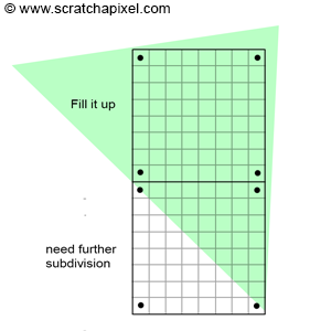
Another technique to speed up rasterization involves rendering blocks of pixels. Instead of testing every pixel within a block, we begin by examining the pixels at the block's corners. GPU algorithms might use blocks of 8x8 pixels. This method is part of a more complex concept involving tiles, which we won't delve into here. If all four corners of the 8x8 grid cover the triangle, it's likely that the remaining pixels within the block also cover the triangle, as illustrated in Figure 7. In such cases, testing the other pixels becomes unnecessary, saving considerable time. These pixels can simply be filled with the triangle's colors. If vertex attributes need to be interpolated across the pixel block, this process is also simplified. Having computed them at the corners of the block, you only need to interpolate them linearly in both directions (horizontally and vertically). This optimization proves most effective for triangles that appear large on the screen. Smaller triangles don't benefit as much from this approach.

Optimizing the Edge Function

The edge function can also be optimized. Let's revisit its implementation:

int orient2d(const Point2D& a, const Point2D& b, const Point2D& c)
{
    return (b.x - a.x) * (c.y - a.y) - (b.y - a.y) * (c.x - a.x);
}

Remember, a and b in this function represent the triangle's vertices, and c denotes the pixel coordinates (in raster space). An interesting observation is that this function is called for each pixel within the triangle's bounding box. While iterating over multiple pixels, only c changes; a and b remain constant. Suppose we calculate the equation once and obtain a result w0:

w0 = (b.x - a.x) * (c.y - a.y) - (b.y - a.y) * (c.x - a.x);

If c.x increases by a step s (the per pixel increment), the new value of w0 becomes:

w0_new = (b.x - a.x) * (c.y - a.y) - (b.y - a.y) * (c.x + s - a.x);

By subtracting the original equation from the new one, we find:

w0_new - w0 = -(b.y - a.y) * s;

Since -(b.y - a.y) * s is constant for a specific triangle (given that s is a consistent increment and a and b are constant), we can calculate it once and store it as w0_step. This simplifies the calculation to:

w0_new = w0 + w0_step;

This adjustment can also be applied to w1 and w2, as well as for steps in c.y.

Originally, the edge function requires 2 multiplications and 5 subtractions, but with this optimization, it can be reduced to a simple addition, although initial values must be computed. This technique is widely discussed online. While we won't use it in this lesson, we plan to explore it further and implement it in a future lesson dedicated to advanced rasterization techniques.

Fixed Point Coordinates

To conclude this section, let's briefly discuss the technique of converting vertex coordinates from floating-point to fixed-point format just before the rasterization stage. "Fixed-point" is the technical term for what is essentially integer representation. When vertex coordinates are converted from NDC to raster space, they are also transformed from floating-point numbers to fixed-point numbers. Why do we do this? The answer isn't straightforward, but in essence, GPUs utilize fixed-point arithmetic because handling integers, through logical bit operations, is computationally easier and faster than dealing with floats or doubles. This explanation is quite generalized; the transition from floating-point to integer coordinates and the implementation of rasterization using integer coordinates encompass a broad and complex topic scarcely documented online, which is surprising given its central role in modern GPU functionality.

This conversion involves rounding vertex coordinates to the nearest integer. However, doing only this could align vertex coordinates too closely with pixel corners, a minor issue for still images but one that creates visual artifacts in animations (vertices may align with different pixels frame by frame). The solution involves converting the number to the smallest integer value while also reserving some bits to represent the sub-pixel position of the vertex (the vertex position's fractional part). Typically, GPUs allocate 4 bits for sub-pixel precision. For a 32-bit integer, 1 bit might be used for the number's sign, 27 bits for the vertex's integer position, and 4 bits for the vertex's fractional position within the pixel. This arrangement implies that the vertex position is "aligned" to the nearest corner of a 16x16 sub-pixel grid, as illustrated in Figure 8. Although vertices are still snapped to a grid, this method is less problematic than aligning them to pixel coordinates. This process introduces other challenges, including integer overflow, which can occur because integers represent a narrower range of values than floats. Additionally, integrating anti-aliasing adds complexity. Thoroughly exploring this topic would require its own lesson.

Fixed-point coordinates expedite the rasterization process and edge function calculations. This efficiency is a key reason for converting vertex coordinates to integers, a technique that will be further discussed in an upcoming lesson.

Notes Regarding Our Implementation of the Rasterization Algorithm

We'll now briefly review the code provided in the source code chapter, highlighting its main components:

• We use the function computeScreenCoordinates to determine the screen coordinates, following the method outlined in the lesson on the pinhole camera model. This ensures our render output is comparable to renders from Maya, which also employs a physically-based camera model.

  float t, b, l, r; 
  
  computeScreenCoordinates( 
      filmApertureWidth, filmApertureHeight, 
      imageWidth, imageHeight, 
      kOverscan, 
      nearClippingPlane, 
      focalLength, 
      t, b, l, r); 
  

• The convertToRaster function transitions triangle vertex coordinates from camera space to raster space, akin to the computePixelCoordinates function from a previous lesson. Remember, we learned a method for converting screen space coordinates to NDC space (where coordinates range between [-1,1] in the GPU realm). We apply the same remapping method here. An important distinction from earlier lessons is that projected points must now be 3D points, with their x- and y-coordinates representing the projected point in screen space and the z-coordinate reflecting the vertex's camera space z-coordinate. This z-coordinate is crucial for addressing visibility issues as explained in chapter four.

  convertToRaster(v0, worldToCamera, l, r, t, b, nearClippingPlane, imageWidth, imageHeight, v0Raster); 
  convertToRaster(v1, worldToCamera, l, r, t, b, nearClippingPlane, imageWidth, imageHeight, v1Raster); 
  convertToRaster(v2, worldToCamera, l, r, t, b, nearClippingPlane, imageWidth, imageHeight, v2Raster);
  

• Remember, all vertex attributes associated with triangle vertices also need "pre-division" by the vertices' z-coordinates for perspective-correct interpolation. This typically occurs just before rendering the triangle (immediately before the pixel iteration loop). However, in the code, the vertex z-coordinate is set to its reciprocal (to expedite depth computation using multiplication instead of division).

  // Precompute reciprocal of the vertex z-coordinate
  v0Raster.z = 1 / v0Raster.z, 
  v1Raster.z = 1 / v1Raster.z, 
  v2Raster.z = 1 / v2Raster.z; 
  
  Vec2f st0 = st[stindices[i * 3]]; 
  Vec2f st1 = st[stindices[i * 3 + 1]]; 
  Vec2f st2 = st[stindices[i * 3 + 2]]; 
  
  // Needed for perspective-correct interpolation
  st0 *= v0Raster.z, st1 *= v1Raster.z, st2 *= v2Raster.z;
  

• The function encompasses two loops: an outer loop iterating over all scene triangles and an inner loop covering all pixels within the bounding box overlapping the current triangle. Notably, some variables in the inner loop are constants and thus can be pre-computed, including the triangle vertices' z-coordinates inverse, linearly interpolated for each pixel covering the triangle (as well as vertex attributes requiring division by their respective z-coordinates).

  // Outer loop: Loop over triangles
  for (uint32_t i = 0; i < ntris; ++i) {
      ...
      // Inner loop: Loop over pixels
      for (uint32_t y = y0; y <= y1; ++y) { 
          for (uint32_t x = x0; x <= x1; ++x) {
              ...
          }
      }
  }
  

• Each pixel undergoes a coverage test using the edge function technique. If a pixel covers a triangle, we compute its barycentric coordinates and then determine the sample depth. Passing the depth buffer test allows us to update the buffer with the new depth value and the frame buffer with the triangle color.

  Vec3f pixelSample(x + 0.5, y + 0.5, 0); 
  float w0 = edgeFunction(v1Raster, v2Raster, pixelSample); 
  float w1 = edgeFunction(v2Raster, v0Raster, pixelSample); 
  float w2 = edgeFunction(v0Raster, v1Raster, pixelSample); 
  if (w0 >= 0 && w1 >= 0 && w2 >= 0) { 
      w0 /= area; 
      w1 /= area; 
      w2 /= area; 
      // Linearly interpolate sample depth
      float oneOverZ = v0Raster.z * w0 + v1Raster.z * w1 + v2Raster.z * w2; 
      float z = 1 / oneOverZ; 
      // Pass the depth buffer test?
      if (z < depthBuffer[y * imageWidth + x]) { 
          depthBuffer[y * imageWidth + x] = z;
          // Update frame buffer
          ...
      }
  }
  

• Shading Techniques: To enhance visual interest, we employ several shading methods. The model has one vertex attribute: st or texture coordinates. These coordinates can create a checkerboard pattern, combined with a simple shading technique called facing ratio. The facing ratio is the dot product between the triangle normal (computed via a cross product between two triangle edges) and the view direction. The view direction is the vector from a point P on the triangle being shaded to the camera position E. In camera space, where all points are now defined, the camera position is simply E=(0,0,0), making the view direction -P, which must then be normalized. Since the dot product can be negative, we clamp it to positive values only.

  Vec3f n = (v1Cam - v0Cam).crossProduct(v2Cam - v0Cam); 
  n.normalize(); 
  Vec3f viewDirection = -pt; 
  viewDirection.normalize(); 
  // Facing ratio 
  float nDotView =  std::max(0.f, n.dotProduct(viewDirection));
  

  This technique requires computing the coordinates of P, the point on the triangle overlapped by the pixel, like any other vertex attribute. We take the vertices in camera space, divide them by their z-coordinate, interpolate them with barycentric coordinates, and multiply the result by the sample depth (also coincidentally P's z-coordinate):

  // Get triangle vertices in camera space.
  Vec3f v0Cam, v1Cam, v2Cam; 
  worldToCamera.multVecMatrix(v0, v0Cam); 
  worldToCamera.multVecMatrix(v1, v1Cam); 
  worldToCamera.multVecMatrix(v2, v2Cam); 
  
  // Divide by the respective z-coordinate as with any other vertex attribute and interpolate using 
  // barycentric coordinates.
  float px = (v0Cam.x/-v0Cam.z) * w0 + (v1Cam.x/-v1Cam.z) * w1 + (v2Cam.x/-v2Cam.z) * w2; 
  float py = (v0Cam.y/-v0Cam.z) * w0 + (v1Cam.y/-v1Cam.z) * w1 + (v2Cam.y/-v2Cam.z) * w2; 
   
  // P in camera space
  Vec3f pt(px * z, py * z, -z);
  

• Frame Buffer Output: Finally, the frame buffer's contents are saved in a PPM file, showcasing the rendering results.

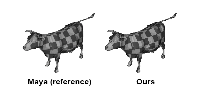
As illustrated, rendering isn't mystical. Understanding the rules allows replication of professional application outputs.

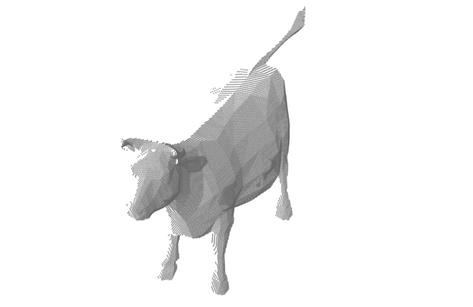
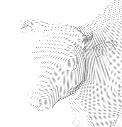
As an additional insight, we exported the world space position of the point on the triangle each image pixel overlaps, displaying all points in a 3D viewer. Unsurprisingly, points appear only on object parts directly visible to the camera, affirming the effectiveness of the depth-buffer technique. The second image provides a close-up of the same point set (right).

Conclusion

Rasterization's main advantages are its simplicity and speed, albeit primarily useful for addressing visibility issues. Remember, rendering involves two steps: visibility and shading. This algorithm offers no shading solutions.

This lesson aims to provide an in-depth introduction to rasterization. If you found this content enlightening and educational, consider supporting our work.

Exercises

• Implement anti-aliasing by dividing the pixel into 4 sub-pixels, generating a sample in the middle of each, conducting the coverage test for each sample, summing the color of the samples, dividing by 4, and setting the pixel color to the result.

• Implement back-face culling by not rendering triangles if the dot product between their normal and the view direction is below a certain threshold. This uses the principle that vectors pointing in opposite directions have a negative dot product. The dot product between two vectors is the cosine of the angle between them. Express the threshold as an angle in degrees.

• Output the content of the z-buffer to a PPM file, remapping depth buffer values to the range [0,255].

Reference

• "A Parallel Algorithm for Polygon Rasterization" by Juan Pineda, Siggraph 1988.

• "A Subdivision Algorithm for Computer Display of Curved Surfaces" by Edwin Earl Catmull, Thesis 1974.

• "Fundamentals of Texture Mapping and Image Warping" by Paul S. Heckbert, Thesis 1989.