The Rasterization Stage
Reading time: 42 mins.Rasterization: What Are We Trying to Solve?
Rasterization is the process by which a primitive is converted to a two dimensional image. Each point of this image contains such information as color and depth Thus rasterizing a primitive consists of two parts The first is to determine which squares of an integer grid in window coordinates are occupied by the primitive The second is assigning a color and a depth value to each such square.
Quote from Chapter 3 of the OpenGL Specification (Version 1.0) document, written by Mark Segal, Kurt Akeley, and Chris Frazier in 1994.
To avoid potential confusion, let me define "rasterization": For our present purposes, it's the process of determining which pixels are inside a triangle, and nothing more.
Michael Abrash, 2009.
In the previous chapter, we learned how to perform the first step of the rasterization algorithm, which is projecting the triangle from 3D space onto the canvas. However, this description isn't entirely accurate. In fact, what we did was transform the triangle from camera space to screen space, which, as mentioned earlier, is also a three-dimensional space. The x- and y-coordinates of the vertices in screen space (let's call them \(VProj\)) correspond to the positions of the triangle vertices on the canvas (let's call them \(V\)). By converting them from screen space to NDC (Normalized Device Coordinates) space and then finally from NDC space to raster space, we obtain the following:
-
The x and y coordinates of \(VProj\) store the coordinates of the \(V\) vertices in raster space (in other words, their projected coordinates onto the screen).
-
The z coordinate of \(VProj\) stores the original \(V\) z-coordinate, negated so that we work with positive numbers instead of negative ones.
In this way, you can think of \(VProj\) as being a 3D point.
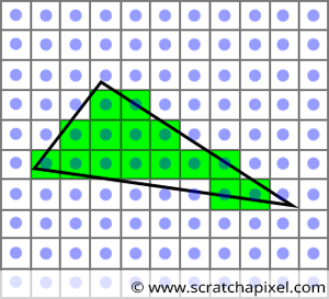
What we need to do next is to loop over the pixels in the image and find out if any of these pixels overlap the "projected image" of the triangle (Figure 1).
When I read this lesson in 2024, many years after writing the first version of it in 2012, I found myself confused by my own wording, particularly with the concept of a pixel overlapping a triangle. Twelve years later, I wondered if it might be less confusing for readers to think of it the other way around—saying that the triangle overlaps the pixel. However, the key idea—and it's helpful if you can mentally picture this—is to imagine projecting a 3D triangle onto the surface of the screen, and then looking at individual pixels in the image to see if they effectively overlap that projected triangle. In this context, thinking of the pixel as overlapping the triangle does make some sense, so I decided to stick with that terminology for the remainder of this lesson. However, I've added this clarification and the small illustration below to help you visualize the process more clearly.

Now, it's a bit more complicated than that (of course!), because what we're actually checking is whether the point located at the center of the pixel (called the sample) is contained within the boundaries of the projected triangle. So, we're not really considering the pixel as a surface and checking whether the entire surface of the projected triangle is "covered" by the pixel. Instead, we're checking if the point at the center of the pixel is within the edges of the projected triangle. This is the test we'll be learning about in this chapter.
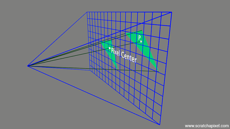
However (yes, it gets more complicated), remember that a pixel is essentially a small window onto the 3D scene. You can think of a pixel as if you were looking at the outside landscape through a real window. Through that window, the triangle might appear to completely cover the pixel's surface or only partially cover it. In an ideal scenario, what would be visible through that pixel window would be a perfect image of the scene. If you consider the image below, what we would ideally like is for the content of the pixel to represent what we see through the window on the right. Of course, we've chosen a simple example on the left, where the scene contains a single triangle, and that triangle covers the entire surface of the pixel. So it's not a problem in this case, but imagine a situation in which several triangles would be visible through that pixel, or a scene like the one visible in the right image.
However, because a pixel is just a single element capable of storing only one color, we can't capture an entire image of what's visible through the window within the pixel. We can only store a single color. So, what we do is sample the color visible at the center of the window. In short, we represent what's visible through the "pixel" window by the color visible at the center of that window. We sample the scene with a single sample, which gives us a single color to store as the pixel's color.
An astute reader might ask, "What if multiple triangles of different colors are visible through that window, and the triangle that projects to the center of the pixel window isn't representative of the others (maybe it's much smaller or only partially visible)? What if the sample in the middle 'misses' it, as shown in the figure below?"

That's an excellent question. You've just identified one of the most critical limitations of digital imaging technology: it forces us to discretize a world that is essentially made of continuous surfaces. This causes a lot of issues related to sampling theory. We won't dive into that topic now, but it's important that you're aware of this limitation and have a clear understanding of the process and its key constraints.
One way to alleviate the problem you've identified is by considering multiple samples per pixel, a technique called multi-sampling. This approach helps represent situations more accurately where triangles partially overlap the pixel's window. Here, we're talking about coverage, a term you'll often encounter in GPU technology. If more than one triangle is visible through the window, using multiple samples increases the likelihood of capturing the various colors visible through the pixel. By averaging these colors, the final pixel color more accurately represents the overall image of the scene as seen through that pixel. Of course, the more samples you use, the slower it takes to render the image. However, in reality, GPUs, especially those specialized for the rasterization algorithm, have ways to make the cost of using, say, 4 samples almost negligible by leveraging the mathematical properties of the rasterization process itself.

With these clarifications made (I didn't realize when I asked myself whether writing that the pixel overlaps the triangle was effectively okay, that it would lead me this far), let's get back to the rasterization process.
Remember, the goal now is to loop over the pixels in the image and determine if any of these pixels (or more precisely, the point at the center of a pixel, as explained earlier) overlaps the "projected image" of the triangle. In graphics API specifications, this test is sometimes called the inside-outside test or the coverage test. The term "coverage" stems from early rasterization algorithms, such as the one used in Pixar's original PRMAN renderer, which tracked the area covered by each individual triangle inside a pixel.
If a pixel overlaps the triangle, we set the pixel in the image to the triangle's color (green in the example from Figure 1). The concept is straightforward, but we now need a method to determine whether a given pixel overlaps a triangle. This is what we will explore in this chapter.
The method typically used in rasterization to solve this problem involves a technique known as the edge function. This function also provides valuable information about the position of the pixel within the projected image of the triangle, known as barycentric coordinates. Barycentric coordinates play an essential role in calculating the actual depth (or the z-coordinate) of the point on the surface of the triangle that the pixel overlaps in 3D (camera) space. In other words, the point's \(P\) z-coordinate (image below). In this chapter, we will also explain what barycentric coordinates are and how they are calculated.
At the end of this chapter, you will be able to produce a very basic rasterizer. In the next chapter, we will look into the possible issues with this very naive implementation of the rasterization algorithm. We will list what these issues are as well as study how they are typically addressed.
While real implementations, whether on GPU or CPU, are highly optimized, this lesson focuses on helping you understand the basic principles of rasterization, not on developing an optimized renderer. Exploring optimizations within the rasterization algorithm is left to you or as a topic for a future lesson.
Keep in mind that drawing a triangle (since the triangle is the primitive we will use in this case) is a two-step problem:
-
Step 1: We first need to find which pixels overlap the triangle.
-
Step 2: We then need to define the colors that the pixels overlapping the triangle should be set to, a process called shading.
The rasterization stage essentially deals with the first step. The reason we say "essentially" rather than "exclusively" is that, during the rasterization stage, we will also compute something called barycentric coordinates, which are to some extent used in the second step. Let's first learn about the edge function (step 1) and then move on to barycentric coordinates and their generation, which are necessary for step 2.
The Edge Function
As mentioned earlier, there are several methods to determine if a pixel (or the point at the center of the pixel) is within a triangle's edges. Although it would be valuable to document older techniques, this lesson will focus on the most commonly used method today. This approach was introduced by Juan Pineda in his 1988 paper titled A Parallel Algorithm for Polygon Rasterization.
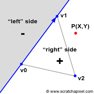
Before delving into Pineda's technique itself, let's first understand the principle behind his method. Imagine the edge of a triangle as a line that splits the 2D plane (the image plane) into two (as shown in Figure 2). The principle of Pineda's method is to find a function, which he called the edge function, so that when we test on which side of this line a given point is (the point P in Figure 2), the function returns a positive number when it is to the right of the line, a negative number when it is to the left of this line, and zero when the point is exactly on the line.
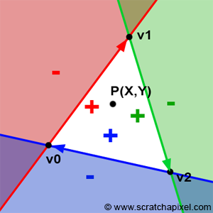
In Figure 2, we applied this method to the first edge of the triangle (defined by the vertices v0 and v1; note that the order is important). If we now apply the same method to the other two edges (v1-v2 and v2-v0), we can see that there is an area (the white triangle) within which all points yield positive results (Figure 3). If we take a point within this area, then we will find that this point is to the right of all three edges of the triangle. If \(P\) is a point in the center of a pixel, we can then use this method to determine if the pixel overlaps or covers the triangle. If for this point, the edge function returns a positive number for all three edges, then the pixel is contained within the triangle (or may lie on one of its edges). The function Pineda uses also happens to be linear, which means that it can be computed incrementally, but we will revisit this point later.
Now that we understand the principle, let's examine the function itself. The edge function is defined as follows (for the edge defined by vertices V0 and V1):
$$E_{01}(P) = (P.x - V0.x) \cdot (V1.y - V0.y) - (P.y - V0.y) \cdot (V1.x - V0.x).$$As the paper mentions, this function has the useful property that its value is related to the position of the point \(P\) relative to the edge defined by the points \(V0\) and \(V1\):
-
\(E(P) > 0\) if \(P\) is to the "right" side
-
\(E(P) = 0\) if \(P\) is exactly on the line
-
\(E(P) < 0\) if \(P\) is to the "left" side
This function is mathematically equivalent to the magnitude of the cross products between the vector \((V1-V0)\) and \((P-V0)\). We can also represent these vectors in matrix form. Presenting them as a matrix serves no other purpose than to neatly display the two vectors:
$$ \begin{vmatrix} (P.x - V0.x) & (P.y - V0.y) \\ (V1.x - V0.x) & (V1.y - V0.y) \end{vmatrix} $$If we denote \(A = (P-V0)\) and \(B = (V1 - V0)\), then we can represent the vectors \(A\) and \(B\) as a 2x2 matrix:
$$ \begin{vmatrix} A.x & A.y \\ B.x & B.y \end{vmatrix} $$The determinant of this matrix can be calculated as:
$$A.x \cdot B.y - A.y \cdot B.x.$$If we substitute the vectors \(A\) and \(B\) back with \((P-V0)\) and \((V1-V0)\), respectively, we obtain:
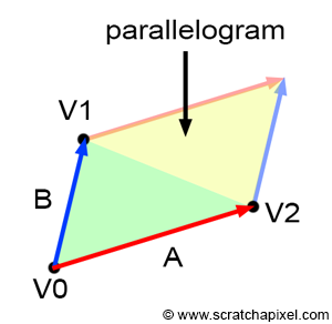
$$(P.x - V0.x) \cdot (V1.y - V0.y) - (P.y - V0.y) \cdot (V1.x - V0.x).$$As you can see, this is similar to the edge function we have defined above. In other words, the edge function can be interpreted either as the determinant of the 2x2 matrix defined by the components of the 2D vectors \((P-V0)\) and \((V1-V0)\), or as the magnitude of the cross product of the vectors \((P-V0)\) and \((V1-V0)\). Both the determinant and the magnitude of the cross product of two vectors have the same geometric interpretation. Let's explain.
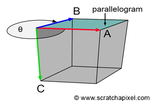
Understanding what happens is easier when we examine the result of a cross-product between two 3D vectors (Figure 4). In 3D, the cross-product returns another 3D vector that is perpendicular (or orthonormal) to the two original vectors. However, as shown in Figure 4, the magnitude of this orthonormal vector depends on the angle between the two vectors. The closer the vectors are to being parallel, the smaller the magnitude, and the closer they are to being perpendicular, the larger the magnitude.
Assuming a right-hand coordinate system, when vectors A (red) and B (blue) are either pointing exactly in the same direction or in opposite directions, the magnitude of the third vector C (green) is zero. Vector A has coordinates (1,0,0) and is fixed. When vector B has coordinates (0,0,-1), the green vector, vector C, has coordinates (0,-1,0). If we calculate its "signed" magnitude, we find that it is equal to -1. Conversely, when vector B has coordinates (0,0,1), vector C has coordinates (0,1,0), and its signed magnitude is equal to 1. In one case, the "signed" magnitude is negative, and in the other, it is positive.
In 3D, the magnitude of a vector can also be interpreted as the area of the parallelogram formed by vectors A and B as sides. This is expressed mathematically using the cross product:
$$\text{Area} = || A \times B ||.$$However, this can also be written as:
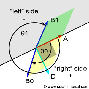
$$\text{Area} = ||A|| \cdot ||B|| \cdot \sin(\theta),$$where \(\theta\) is the angle between the two vectors. The sine function precisely explains the change of sign: when the angle \(\theta\) is between 0 and 180 degrees, the result is positive; when the angle is greater than 180 degrees, the result becomes negative. This relationship is key to understanding how the orientation of vectors affects the direction and sign of the resulting cross product. An area should always be positive, though the sign of the above equation provides an indication of the orientation of vectors A and B with respect to each other. When B is within the half-plane defined by vector A and a vector orthogonal to A (let's call this vector D; note that A and D form a 2D Cartesian coordinate system), then the result of the equation is positive. When B is within the opposite half-plane, the result is negative (Figure 6). Another way to explain this result is that the result is positive when the angle \(\theta\) is in the range \((0,\pi)\) and negative when \(\theta\) is in the range \((\pi, 2\pi)\). Note that when \(\theta\) is exactly equal to 0 or \(\pi\), then the cross-product or the edge function returns 0.
Typically, the notation for exclusive bounds is written using parentheses, like this: (a, b) to indicate that the interval does not include the endpoints a and b. For inclusive bounds in mathematical notation, square brackets are used to indicate that the endpoints are included in the range. For example: \([a, b]\) means the interval includes both \(a\) and \(b\).
To determine if a point is inside a triangle, what really matters is the sign of the function used to compute the area of the parallelogram. However, the area itself also plays a key role in the rasterization algorithm; it is used to compute the barycentric coordinates of the point within the triangle, a technique we will explore next. You're correct that the methods for calculating the area of a parallelogram in 2D and 3D are conceptually similar, and both the cross product and the determinant approach work in both dimensions. The cross-product in 3D and 2D shares the same geometric interpretation: both return the signed area of the parallelogram defined by the two vectors. In 3D, this area is computed using the magnitude of the cross-product:
$$\text{Area} = || A \times B || = ||A|| \cdot ||B|| \cdot \sin(\theta).$$In 2D, the area can also be calculated using the cross-product, which is equivalent to the determinant of a 2x2 matrix:
$$\text{Area} = A.x \cdot B.y - A.y \cdot B.x.$$Both methods effectively calculate the area of the parallelogram in their respective dimensions, with the determinant approach in 2D providing the signed area directly. The key difference is that in 3D, the cross-product results in a vector whose magnitude gives the area, while in 2D, the result is a scalar that directly represents the signed area.
From a practical standpoint, all we need to do now is test the sign of the edge function for each edge of the triangle and another vector defined by a point and the first vertex of the edge being tested (Figure 7).
$$ \begin{array}{l} E_{01}(P) = (P.x - V0.x) \cdot (V1.y - V0.y) - (P.y - V0.y) \cdot (V1.x - V0.x),\\ E_{12}(P) = (P.x - V1.x) \cdot (V2.y - V1.y) - (P.y - V1.y) \cdot (V2.x - V1.x),\\ E_{20}(P) = (P.x - V2.x) \cdot (V0.y - V2.y) - (P.y - V2.y) \cdot (V0.x - V2.x). \end{array} $$If all three tests are positive or equal to 0, then the point is inside the triangle (or lying on one of its edges). If any one of the tests is negative, then the point is outside the triangle. In code, we have:
bool edgeFunction(const Vec2f &a, const Vec3f &b, const Vec2f &c) {
    return ((c.x - a.x) * (b.y - a.y) - (c.y - a.y) * (b.x - a.x) >= 0);
}

bool inside = true;
inside &= edgeFunction(V0, V1, p);
inside &= edgeFunction(V1, V2, p);
inside &= edgeFunction(V2, V0, p);

if (inside) {
    // point p is inside the triangle defined by vertices V0, V1, V2
    ...
}
The edge function has the property of being linear. We refer you to the original paper if you wish to learn more about this property and how it can be used to optimize the algorithm. In short, because of this property, the edge function can be run in parallel (several pixels can be tested at once), making the method ideal for hardware implementation. This partially explains why pixels on the GPU are generally rendered as a block of 2x2 pixels (enabling pixels to be tested in a single cycle). Hint: You can also use SSE instructions and multi-threading to optimize the algorithm on the CPU.
Alternative to the Edge Function
There are alternative methods to the edge function for determining if pixels overlap triangles. However, as mentioned in the introduction of this chapter, we won't explore them in this lesson. For reference, another common technique is scanline rasterization, based on the Bresenham algorithm, generally used for drawing lines. GPUs mostly use the edge method because it is more generic and easier to parallelize than the scanline approach, but further details on this topic will not be provided in this lesson.
Winding: Vertex Ordering Matters
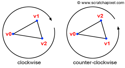
One aspect we haven't discussed yet, but which holds great importance in 3D rendering in general, is the order in which the vertices that make up the triangles are defined. There are two possible options, illustrated in Figure 8: clockwise or counter-clockwise ordering. This ordering is also referred to do as winding. Winding is crucial because it essentially defines one important property of the triangle: which side of the triangle is considered as the front face, which in tirns defines the triang'e normal orientation. Remember, the normal of the triangle can be computed from the cross product of two vectors, \(A=(V2-V0)\) and \(B=(V1-V0)\). Suppose \(V0=\{0,0,0\}\), \(V1=\{1,0,0\}\), and \(V2=\{0,-1,0\}\), then \((V1-V0)=\{1,0,0\}\) and \((V2-V0)=\{0,-1,0\}\). Now, let's compute the cross product of these two vectors:
$$ \begin{array}{l} N = (V1-V0) \times (V2-V0)\\ N.x = a.y \cdot b.z - a.z \cdot b.y = 0 \cdot 0 - 0 \cdot -1\\ N.y = a.z \cdot b.x - a.x \cdot b.z = 0 \cdot 0 - 1 \cdot 0\\ N.z = a.x \cdot b.y - a.y \cdot b.x = 1 \cdot -1 - 0 \cdot 0 = -1\\ N=\{0,0,-1\} \end{array} $$However, if you declare the vertices in counter-clockwise order, with \(V0=\{0,0,0\}\), \(V1=\{0,-1,0\}\), and \(V2=\{1,0,0\}\), \((V1-V0)=\{0,-1,0\}\) and \((V2-V0)=\{1,0,0\}\)and calculate the cross-product of these two vectors we get:
$$ \begin{array}{l} N = (V1-V0) \times (V2-V0)\\ N.x = a.y \cdot b.z - a.z \cdot b.y = 0 \cdot 0 - 0 \cdot -1\\ N.y = a.z \cdot b.x - a.x \cdot b.z = 0 \cdot 0 - 1 \cdot 0\\ N.z = a.x \cdot b.y - a.y \cdot b.x = 0 \cdot 0 - -1 \cdot 1 = 1\\ N=\{0,0,1\} \end{array} $$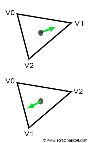
As expected, the two normals point in opposite directions. The orientation of the normal is crucial for several reasons, one of the most important being face culling. Most rasterizers, and even ray tracers, may not render triangles whose normals face away from the camera, a process known as back-face culling. Most rendering APIs, such as OpenGL or DirectX, allow back-face culling to be turned off. However, it's still important to be aware that vertex ordering affects rendering outcomes, among other factors. Surprisingly, the edge function is also affected by vertex ordering. It's worth noting that there's no universal rule for choosing the order. Many details in a renderer's implementation can change the normal's orientation, so you can't assume that declaring vertices in a certain order guarantees the normal will face a specific direction. For instance, using vectors \(A=(V0-V1)\) and \(B=(V2-V1)\) could produce the same normal but flipped. Even using \(A=(V1-V0)\) and \(B=(V2-V0)\), the order of vectors in the cross-product (\(A \times B = -B \times A\)) also affects the normal's direction. For these reasons, assuming a specific outcome based on vertex order is unreliable. What's important is adhering to the chosen convention. Generally, graphics APIs like OpenGL, Vulkan, or DirectX expect triangles to be declared in counterclockwise order, which we will also adopt. Both parameters—winding order and whether you want to render the front or back face of the triangle, or both—can be specified through their respective APIs, generally using parameters called FrontFace with two modes, FRONT_FACE_COUNTER_CLOCKWISE and FRONT_FACE_CLOCKWISE for the ordering, and CullMode, which can be set to NONE, CULL_MODE_FRONT, CULL_MODE_BACK, or CULL_MODE_FRONT_AND_BACK.
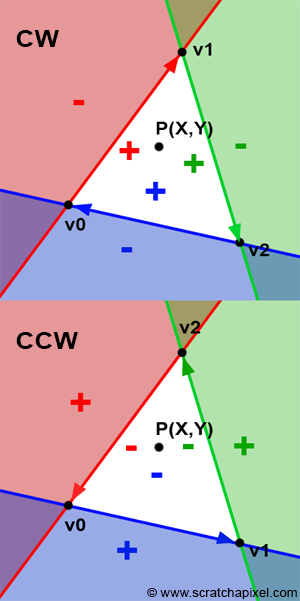
Why does winding matter when it comes to the edge function? You may have noticed that, since the beginning of this chapter, we have drawn the triangle vertices in clockwise order. We have also defined the edge function as:
$$ \begin{array}{l} E_{AB}(P) &= (P.x - A.x) \cdot (B.y - A.y) - \\ & (P.y - A.y) \cdot (B.x - A.x) \end{array} $$If we adhere to this convention, then points to the right of the line defined by vertices A and B will be positive. For example, a point to the right of \(V0V1\), \(V1V2\), or \(V2V0\) would be positive. However, if we were to declare the vertices in counterclockwise order, points to the right of an edge defined by vertices \(A\) and \(B\) would still be positive, but they would be outside the triangle. In other words, points contained within the triangle would not be positive but negative (Figure 10). You can still make the code work with positive numbers by adjusting the edge function as follows:
$$ E_{AB}(P) = (A.x - B.x) \cdot (P.y - A.y) - (A.y - B.y) \cdot (P.x - A.x). $$In conclusion, you may need to use one version of the edge function or the other depending on the winding convention you follow.
Barycentric Coordinates
Computing barycentric coordinates is not necessary for the rasterization algorithm to work. In a basic implementation of the rendering technique (to generate an image of a triangle or several triangles), all you need to do is project the vertices and use a technique like the edge function we described earlier to determine if pixels are contained within the projected triangle's edges. These are the only two essential steps to produce an image. While this is an accomplishment, it only allows us to generate images of triangles filled with uniform colors. But what if we want the color to vary across the surface of the triangles? What about shading in general?
The result of the edge function, which can be interpreted as the area of the parallelogram defined by vectors A and B, can also be used to calculate the barycentric coordinates we've mentioned before. How convenient! We can use the result of the edge function for two purposes: testing points inside a triangle and calculating the barycentric coordinates, which, as you might have guessed, will be crucial for shading the triangles.
Before we go any further, let's explain what barycentric coordinates are. First, they come in a set of three floating-point numbers which, in this lesson, we will denote \(\lambda_0\), \(\lambda_1\), and \(\lambda_2\). Many different conventions exist, but Wikipedia uses the Greek letter lambda (\(\lambda\)), which is also used by other authors (the Greek letter omega (\(\omega\)) is also sometimes used). This doesn't matter; you can call them whatever you want. In short, the coordinates can be used to define any point on the triangle in the following manner:
$$P = \lambda_0 \cdot V0 + \lambda_1 \cdot V1 + \lambda_2 \cdot V2.$$Where, as usual, \(V0\), \(V1\), and \(V2\) are the vertices of a triangle. These coordinates can take on any value, but for points that are inside the triangle (or lying on one of its edges), they must be within the range \([0, 1]\), and the sum of the three coordinates must equal 1. In other words:
$$\lambda_0 + \lambda_1 + \lambda_2 = 1, \text{ for } P \in \triangle{V0, V1, V2}.$$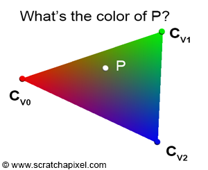
This equation, \(P = \lambda_0 \cdot V0 + \lambda_1 \cdot V1 + \lambda_2 \cdot V2\), is a form of interpolation, if you will. A point overlapping the triangle can be defined as "a little bit of V0, plus a little bit of V1, plus a little bit of V2." Note that when any of the coordinates is 1 (which means the others must be 0), the point \(P\) is equal to one of the triangle's vertices. For example, if \(\lambda_2 = 1\), then \(P\) is equal to \(V2\). This is why barycentric coordinates are sometimes referred to as weights for the triangle's vertices (which is why in the code, we denote them with the letter \(w\)).
While interpolating the triangle's vertices to find the position of a point inside the triangle may not seem very useful initially (though we will eventually need this information when we consider shading more seriously, as both the point on the triangle and the normal at that point are key variables in the shading process), the method becomes truly valuable for shading. It can be used to interpolate any variable defined at the triangle's vertices across the surface of the triangle. For example, imagine you have defined a color at each vertex of the triangle: \(V0\) is red, \(V1\) is green, and \(V2\) is blue (Figure 12). You want to determine how these three colors are interpolated across the surface of the triangle at point \(P\) (the sampled point). If you know the barycentric coordinates of this point \(P\), then its color \(C_P\) (which is a combination of the triangle vertices' colors) is defined as:
$$C_P = \lambda_0 \cdot C_{V0} + \lambda_1 \cdot C_{V1} + \lambda_2 \cdot C_{V2}.$$This technique proves very useful for shading triangles. Data associated with the vertices of triangles, called vertex attributes, is a common and important technique in computer graphics (CG). The most common vertex attributes include colors, normals, and texture coordinates. Practically, this means that when you define a triangle, you don't only pass the triangle's vertices to the renderer but also its associated vertex attributes. For example, to shade the triangle, you may need color and normal vertex attributes, which means each triangle will be defined by 3 points (the triangle vertex positions), 3 colors (the colors of the triangle vertices), and 3 normals (the normals of the triangle vertices). Normals too can be interpolated across the surface of the triangle. Interpolated normals are used in a technique called smooth shading, first introduced by Henri Gouraud. We will explore this technique later when we discuss shading.
How do we find these barycentric coordinates? It turns out to be straightforward. As mentioned earlier when introducing the edge function, the result of the edge function can be interpreted as the area of the parallelogram defined by vectors \(A\) and \(B\). If you examine Figure 8, you'll notice that the area of the triangle defined by vertices \(V0\), \(V1\), and \(V2\) is just half the area of the parallelogram formed by vectors \(A\) and \(B\). Therefore, the area of the triangle is half the area of the parallelogram, which, as we know, can be computed using the cross-product of the two 2D vectors \(A\) and \(B\):
$$Area_{\triangle{V0V1V2}}= \frac{1}{2} \times (A \times B) = \frac{1}{2} \times (A.x \cdot B.y - A.y \cdot B.x).$$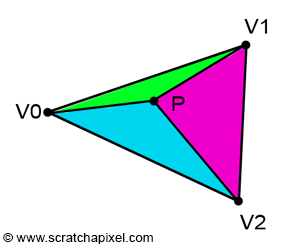
If point P is inside the triangle, then, as illustrated in Figure 3, we can draw three sub-triangles: \(V0-V1-P\) (green), \(V1-V2-P\) (magenta), and \(V2-V0-P\) (cyan). It is clear that the sum of these three sub-triangle areas is equal to the area of the triangle \(V0-V1-V2\):
$$ \begin{array}{l} Area_{\triangle{V0V1V2}} = Area_{\triangle{V0V1P}} + \\ Area_{\triangle{V1V2P}} + \\ Area_{\triangle{V2V0P}}. \end{array} $$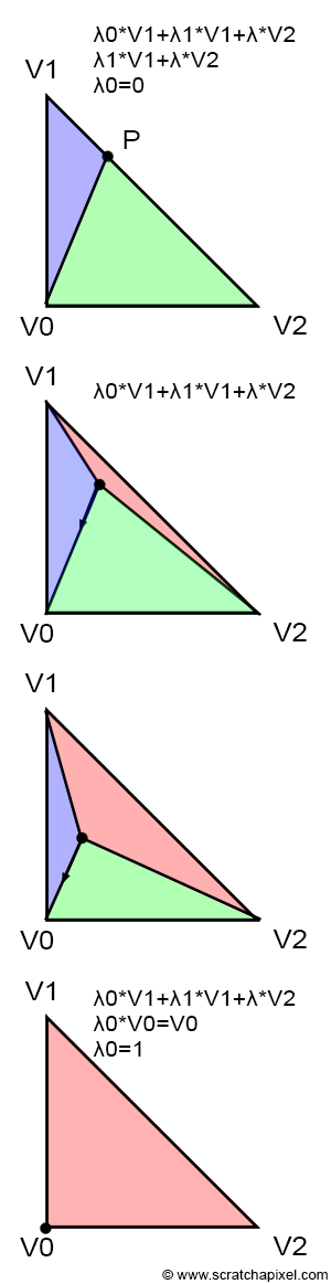
Let's first intuitively understand how they work, which might be easier if you look at Figure 14. Each image in the series shows what happens to the sub-triangle as point \(P\), originally on the edge defined by vertices \(V1-V2\), moves towards \(V0\). Initially, P lies exactly on the edge \(V1-V2\). This scenario is akin to basic linear interpolation between two points. In other words, we could write:
$$P = \lambda_1 \cdot V1 + \lambda_2 \cdot V2$$With \(\lambda_1 + \lambda_2 = 1\), thus \(\lambda_2 = 1 - \lambda_1\) and \(\lambda_0 = 0\).
Let's recap:
$$ \begin{array}{l} P = \lambda_0 \cdot V0 + \lambda_1 \cdot V1 + \lambda_2 \cdot V2,\\ P = 0 \cdot V0 + \lambda_1 \cdot V1 + \lambda_2 \cdot V2,\\ P = \lambda_1 \cdot V1 + \lambda_2 \cdot V2.\\ P = \lambda_1 \cdot V1 + (1- \lambda_1) \cdot V2. \end{array} $$This is relatively straightforward. Also, note that in the first image, the red triangle is not visible, and that \(P\) is closer to \(V1\) than to \(V2\). Therefore, \(\lambda_1\) is necessarily greater than \(\lambda_2\). Furthermore, the green triangle is larger than the blue triangle. To summarize: the red triangle is not visible when \(\lambda_0 = 0\), the green triangle is larger than the blue triangle, and \(\lambda_1\) is greater than \(\lambda_2\). This suggests a relationship between the areas of the triangles and the barycentric coordinates. Moreover, the red triangle appears to be associated with \(\lambda_0\), the green triangle with \(\lambda_1\), and the blue triangle with \(\lambda_2\):
-
\(\lambda_0\) is proportional to the area of the red triangle,
-
\(\lambda_1\) is proportional to the area of the green triangle,
-
\(\lambda_2\) is proportional to the area of the blue triangle.
Jumping directly to the last image, where \(P\) equals \(V0\), this situation can only occur if \(\lambda_0\) equals 1 and the other two coordinates equal 0:
$$ \begin{array}{l} P = \lambda_0 \cdot V0 + \lambda_1 \cdot V1 + \lambda_2 \cdot V2,\\ P = 1 \cdot V0 + 0 \cdot V1 + 0 \cdot V2,\\ P = V0. \end{array} $$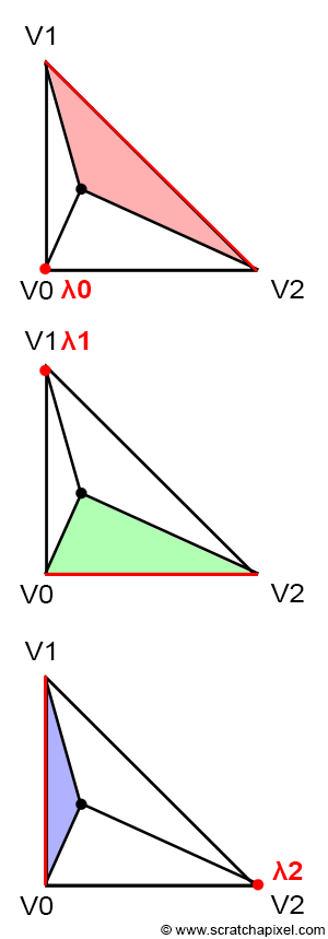
In this specific scenario, the blue and green triangles have disappeared, and the area of the triangle \(V0-V1-V2\) is the same as the area of the red triangle. This confirms our intuition about the relationship between the areas of the sub-triangles and the barycentric coordinates. From the observations above, we can also deduce that each barycentric coordinate is related to the area of the sub-triangle defined by the edge directly opposite the associated vertex and the point \(P\). In other words (see Figure 15):
-
\(\color{red}{\lambda_0}\) is associated with \(V0\). The edge opposite \(V0\) is \(V1-V2\), defining the red triangle with \(V1-V2-P\).
-
\(\color{green}{\lambda_1}\) is associated with \(V1\). The edge opposite \(V1\) is \(V2-V0\), defining the green triangle with \(V2-V0-P\).
-
\(\color{blue}{\lambda_2}\) is associated with \(V2\). The edge opposite \(V2\) is \(V0-V1\), defining the blue triangle with \(V0-V1-P\).
The areas of the red, green, and blue triangles are given by the respective edge functions we used earlier to determine if \(P\) is inside the triangle, divided by 2 (recall that the edge function provides the "signed" area of the parallelogram defined by vectors \(A\) and \(B\), where \(A\) and \(B\) can be any of the triangle's three edges):
$$ \begin{array}{l} \color{red}{Area_{tri}(V1,V2,P)} = \dfrac{1}{2}E_{12}(P),\\ \color{green}{Area_{tri}(V2,V0,P)} = \dfrac{1}{2}E_{20}(P),\\ \color{blue}{Area_{tri}(V0,V1,P)} = \dfrac{1}{2}E_{01}(P). \end{array} $$The barycentric coordinates can be computed as the ratio between the area of the sub-triangles and the area of the triangle \(V0V1V2\):
$$ \begin{array}{l} \color{red}{\lambda_0 = \dfrac{Area(V1,V2,P)}{Area(V0,V1,V2)}},\\ \color{green}{\lambda_1 = \dfrac{Area(V2,V0,P)}{Area(V0,V1,V2)}},\\ \color{blue}{\lambda_2 = \dfrac{Area(V0,V1,P)}{Area(V0,V1,V2)}}. \end{array} $$Dividing by the triangle's area normalizes the coordinates. For example, when \(P\) is positioned at \(V0\), the area of the triangle \(V2V1P\) (the red triangle) is the same as the area of the triangle \(V0V1V2\). Thus, dividing one by the other yields 1, which is the value of the coordinate \(\lambda_0\). Since the green and blue triangles' areas are 0 in this case, \(\lambda_1\) and \(\lambda_2\) equal 0, and we get:
$$P = 1 \cdot V0 + 0 \cdot V1 + 0 \cdot V2 = V0,$$which is the expected result.
To compute the area of a triangle, we can use the edge function as mentioned earlier. This method works for both the sub-triangles and the main triangle \(V0V1V2\). However, the edge function returns the area of the parallelogram instead of the triangle's area (Figure 8). But since the barycentric coordinates are computed as the ratio between the sub-triangle area and the main triangle area, we can ignore the division by 2 (this division, present in both the numerator and denominator, cancels out):
$$\lambda_0 = \dfrac{Area_{tri}(V1,V2,P)}{Area_{tri}(V0,V1,V2)} = \dfrac{\frac{1}{2} E_{12}(P)}{\dfrac{1}{2}E_{12}(V0)} = \dfrac{E_{12}(P)}{E_{12}(V0)}.$$Note that \(E_{01}(V2) = E_{12}(V0) = E_{20}(V1) = 2 \cdot Area_{tri}(V0,V1,V2)\).
Let's examine the code implementation. Previously, we computed the edge functions to test if points were inside triangles, simply returning true or false depending on whether the result of the function was positive or negative. To compute the barycentric coordinates, we need the actual result of the edge function. We can also use the edge function to compute the area (multiplied by 2) of the triangle. Here is an implementation that tests if a point \(P\) is inside a triangle and, if so, computes its barycentric coordinates:
float edgeFunction(const Vec2f &a, const Vec3f &b, const Vec2f &c)
{
    return (c.x - a.x) * (b.y - a.y) - (c.y - a.y) * (b.x - a.x);
}

float area = edgeFunction(v0, v1, v2); // Area of the triangle multiplied by 2
float w0 = edgeFunction(v1, v2, p); // Signed area of the triangle v1v2p multiplied by 2
float w1 = edgeFunction(v2, v0, p); // Signed area of the triangle v2v0p multiplied by 2
float w2 = edgeFunction(v0, v1, p); // Signed area of the triangle v0v1p multiplied by 2

// If point p is inside triangles defined by vertices v0, v1, v2
if (w0 >= 0 && w1 >= 0 && w2 >= 0) {
    // Barycentric coordinates are the areas of the sub-triangles divided by the area of the main triangle
    w0 /= area;
    w1 /= area;
    w2 /= area;
}
Let's apply this code to generate an actual image.
We understand that:
$$\lambda_0 + \lambda_1 + \lambda_2 = 1.$$Furthermore, we know that any value across the surface of the triangle can be computed using the equation:
$$Z = \lambda_0 \cdot Z0 + \lambda_1 \cdot Z1 + \lambda_2 \cdot Z2.$$In this instance, the value we interpolate is Z, which can represent anything we choose, such as the z-coordinate of the triangle's vertices in camera space. We can rewrite the first equation as:
$$\lambda_0 = 1 - \lambda_1 - \lambda_2.$$Substituting this equation into the equation for computing Z and simplifying yields:
$$Z = Z0 + \lambda_1(Z1 - Z0) + \lambda_2(Z2 - Z0).$$The terms \(Z1 - Z0\) and \(Z2 - Z0\) can generally be precomputed, which simplifies the computation of Z to two additions and two multiplications. This optimization is worth mentioning because GPUs utilize it, and it's often discussed for essentially this reason.
Interpolate vs. Extrapolate
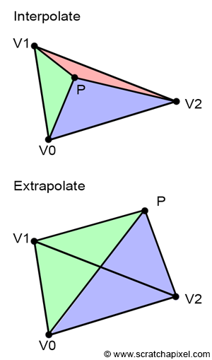
It's important to note that the computation of barycentric coordinates works regardless of the point's position relative to the triangle. In other words, the coordinates are valid whether the point is inside or outside the triangle. When the point is inside, using barycentric coordinates to evaluate the value of a vertex attribute is referred to as interpolation, and when the point is outside, it's called extrapolation. This distinction is crucial because, in some instances, we may need to evaluate the value of a given vertex attribute for points that do not overlap with triangles. Specifically, this is necessary to compute the derivatives of the triangle texture coordinates, which are used for proper texture filtering. If you're interested in delving deeper into this topic, we recommend reading the lesson on Texturing.
For now, remember that barycentric coordinates are valid even when the point doesn't overlap with the triangle, and it's important to understand the difference between vertex attribute extrapolation and interpolation. This will become handy when we will get to the lesson on Texturing.
Rasterization Rules
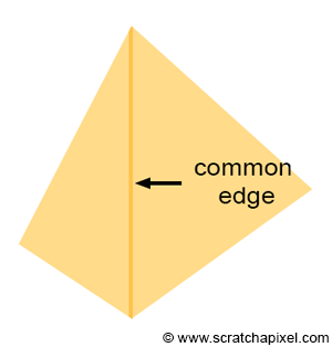
In certain cases, a pixel may overlap more than one triangle, especially when it lies precisely on an edge shared by two triangles, as illustrated in Figure 17. Such a pixel would pass the coverage test for both triangles. If the triangles are semi-transparent, a dark edge may appear where the pixels overlap the two triangles due to the way semi-transparent objects are combined (imagine two superimposed semi-transparent sheets of plastic. The surface becomes more opaque and appears darker than the individual sheets). This phenomenon results in something similar to what is depicted in Figure 18, where a darker line appears where the two triangles share an edge.
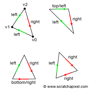
To address this issue, a rule is needed to ensure that a pixel can never overlap two triangles sharing an edge twice. Most graphics APIs, such as OpenGL and DirectX, define what they call the top-left rule. This rule stipulates that a pixel or point is considered to overlap a triangle if it is either inside the triangle or lies on a triangle's top edge or any edge considered to be a left edge. What constitutes a top and left edge? Figure 19 clearly demonstrates the definition of top and left edges.
-
A top edge is an edge that is perfectly horizontal and whose defining vertices are positioned above the third one. Technically, this means that the y-coordinates of the vector V[(X+1)%3]-V[X] are equal to 0, and its x-coordinates are positive (greater than 0).
-
A left edge is essentially an edge that is ascending. Given that vertices are defined in clockwise order in our context, an edge is considered ascending if its respective vector V[(X+1)%3]-V[X] (where X can be 0, 1, 2) has a positive y-coordinate.
If you are using a counter-clockwise order, a top edge is an edge that is horizontal and whose x-coordinate is negative, while a left edge is an edge whose y-coordinate is negative.
In pseudo-code, we have:
// Does it pass the top-left rule?
Vec2f v0 = { ... };
Vec2f v1 = { ... };
Vec2f v2 = { ... };

float w0 = edgeFunction(v1, v2, p);
float w1 = edgeFunction(v2, v0, p);
float w2 = edgeFunction(v0, v1, p);

Vec2f edge0 = v2 - v1;
Vec2f edge1 = v0 - v2;
Vec2f edge2 = v1 - v0;

bool overlaps = true;

// If the point is on the edge, test if it is a top or left edge,
// otherwise test if the edge function is positive
overlaps &= (w0 == 0 ? ((edge0.y == 0 && edge0.x > 0) || edge0.y > 0) : (w0 > 0));
overlaps &= (w1 == 0 ? ((edge1.y == 0 && edge1.x > 0) || edge1.y > 0) : (w1 > 0));
overlaps &= (w2 == 0 ? ((edge2.y == 0 && edge2.x > 0) || edge2.y > 0) : (w2 > 0));

if (overlaps) {
    // The pixel overlaps the triangle.
    ...
}
This version serves as a proof of concept but is highly unoptimized. The fundamental idea is to first check whether any of the values returned by the edge function equals 0, indicating that the point lies on the edge. In such cases, we test if the edge in question is a top-left edge. If it is, it returns true. If the value returned by the edge function is not 0, we then return true if the value is greater than 0. The top-left rule won't be implemented in the program provided with this lesson.
Putting Things Together: Finding if a Pixel Overlaps a Triangle
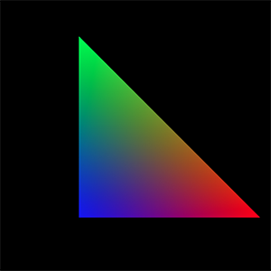
Let's apply the techniques we've learned in this chapter to a program that produces an actual image. We'll assume that the triangle has already been projected (refer to the last chapter of this lesson for a complete implementation of the rasterization algorithm). We will also assign a color to each vertex of the triangle. The process is as follows: we will loop over all the pixels in the image and test if they overlap the triangle using the edge function method. If the edge function returns a positive number for all the edges, then the pixel overlaps the triangle. We can then compute the pixel's barycentric coordinates and use these coordinates to shade the pixel by interpolating the color defined at each vertex of the triangle. The result of the framebuffer is saved to a PPM file (which you can open with Photoshop). The output of the program is shown in Figure 20.
An optimization for this program could involve looping over the pixels contained within the bounding box of the triangle. While this optimization is not implemented in the current version of the program, you are encouraged to try it yourself using the code from the previous chapters. The source code for this lesson is available in the GitHub repository linked at the top of this lesson (at the bottom of the chapter list).
Note that in this version of the program, we move point \(P\) to the center of each pixel. Alternatively, you could use the integer coordinates of the pixel. More details on this topic will be discussed in the next chapter.
// c++ -o raster2d raster2d.cpp
// (c) www.scratchapixel.com

#include <cstdio>
#include <cstdlib>
#include <fstream>

typedef float Vec2[2];
typedef float Vec3[3];
typedef unsigned char Rgb[3];

inline float edgeFunction(const Vec2 &a, const Vec2 &b, const Vec2 &c) {
    return (c[0] - a[0]) * (b[1] - a[1]) - (c[1] - a[1]) * (b[0] - a[0]);
}

int main(int argc, char **argv) {
    Vec2 v0 = {491.407, 411.407};
    Vec2 v1 = {148.593, 68.5928};
    Vec2 v2 = {148.593, 411.407};
    Vec3 c0 = {1, 0, 0};
    Vec3 c1 = {0, 1, 0};
    Vec3 c2 = {0, 0, 1};

    const uint32_t w = 512;
    const uint32_t h = 512;

    Rgb *framebuffer = new Rgb[w * h];
    memset(framebuffer, 0x0, w * h * 3);

    float area = edgeFunction(v0, v1, v2);

    for (uint32_t j = 0; j < h; ++j) {
        for (uint32_t i = 0; i < w; ++i) {
            Vec2 p = {i + 0.5f, j + 0.5f};
            float w0 = edgeFunction(v1, v2, p);
            float w1 = edgeFunction(v2, v0, p);
            float w2 = edgeFunction(v0, v1, p);
            if (w0 >= 0 && w1 >= 0 && w2 >= 0) {
                w0 /= area;
                w1 /= area;
                w2 /= area;
                float r = w0 * c0[0] + w1 * c1[0] + w2 * c2[0];
                float g = w0 * c0[1] + w1 * c1[1] + w2 * c2[1];
                float b = w0 * c0[2] + w1 * c1[2] + w2 * c2[2];
                framebuffer[j * w + i][0] = (unsigned char)(r * 255);
                framebuffer[j * w + i][1] = (unsigned char)(g * 255);
                framebuffer[j * w + i][2] = (unsigned char)(b * 255);
            }
        }
    }

    std::ofstream ofs;
    ofs.open("./raster2d.ppm");
    ofs << "P6\n" << w << " " << h << "\n255\n";
    ofs.write((char*)framebuffer, w * h * 3);
    ofs.close();

    delete [] framebuffer;

    return 0;
}
As you can see, and in conclusion, we can state that the rasterization algorithm is quite straightforward, and its basic implementation is relatively easy as well.
Conclusion and What's Next?
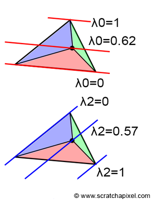
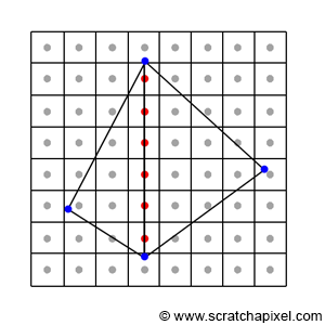
Many fascinating techniques and pieces of trivia are related to the topic of barycentric coordinates, but this lesson serves merely as an introduction to the rasterization algorithm, so we won't delve deeper. However, one interesting piece of trivia to note is that barycentric coordinates remain constant along lines parallel to an edge, as illustrated in Figure 21.
In this lesson, we've explored two important methods and various concepts:
-
Firstly, we learned about the edge function and its application in determining whether a point \(P\) overlaps a triangle. The edge function is calculated for each edge of the triangle, with a second vector defined by the edge's first vertex and the point \(P\). If the function yields a positive result for all three edges, then point \(P\) overlaps the triangle.
-
Additionally, we discovered that the outcome of the edge function can be used to compute the barycentric coordinates of point \(P\). These coordinates allow for the interpolation of vertex data or attributes across the triangle's surface, acting as weights for the triangle's vertices. The most commonly interpolated vertex attributes include color, normals, and texture coordinates.