Ray-Tracing: Rendering a Triangle

Möller-Trumbore algorithm

Möller-Trumbore algorithm

The Möller-Trumbore (or MT for the remainder of this lesson) algorithm is a fast ray-triangle intersection algorithm that was introduced in 1997 by Tomas Möller and Ben Trumbore in a paper titled "Fast, Minimum Storage Ray/Triangle Intersection". It is still considered today a fast algorithm that is often used in benchmarks to compare the performances of other methods. However, a fair comparison of ray-triangle intersection algorithms is difficult because speed can depend on many factors, such as how algorithms are implemented, the type of test scene used, whether values are precomputed, etc.

The Möller-Trumbore algorithm takes advantage of the parameterization of P, the intersection point in barycentric coordinates (which we discussed in the previous chapter). We learned in the previous chapter to calculate P, the intersection point, using the following equation:

We also learned that w=1-u-v; thus, we can write:

If we develop, we get (equation 1):

Note that (B-A) and (C-A) are the edges AB and AC of the triangle ABC. The intersection P can also be written using the ray's parametric equation (equation 2):

Where \(t\) is the distance from the ray's origin to the intersection P. If we replace P in equation 1 with the ray's equation, we get (equation 3):

On the left side of the equal sign, we have three unknowns (t, u, v) multiplied by three known terms (B-A, C-A, D). We can rearrange these terms and present equation 3 using the following notation (equation 4):

The left side of the equation has been rearranged into a row-column vector multiplication. This is the simplest possible form of matrix multiplication. You take the first element of the raw matrix (-D, B-A, C-A) and multiply it by the first element of the column vector (\(t\), \(u\), \(v\)). Then you add the raw matrix's second element multiplied by the column vector's second element. Then finally, add the third element of the raw matrix multiplied by the third element of the column vector (which gives you equation 3 again).

In equation 3, the term on the right side of the equal sign is a vector (O-A). B-A, C-A, and D are vectors as well, and \(t\), \(u\), and \(v\) (unknown) are scalars. This equation is about vectors. It combines three vectors in quantities defined by t, u, and v. It gives another vector as a result of this operation (be aware that in their paper, Möller and Trumbore use the term x-, y- and z-axis instead of \(t\), \(u\) and \(v\) when they explain the geometrical meaning of this equation).

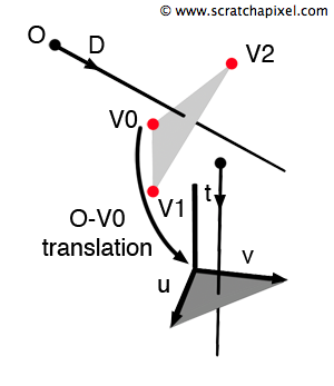
Let's say that P is where the ray intersects the triangle ABC. You will probably agree that the point P Cartesian coordinates (x, y, z) change as we move or rotate the triangle and the ray together. But on the other hand, the barycentric coordinates of P are invariant. If the triangle is rotated, scaled, stretched, or translated, the coordinates u, v defining the position of P with respect to vertices A, B, and C will not change (see Figure 1).

The MT algorithm is taking advantage of this property. Instead of solving the ray-triangle intersection equation using x, y, and z coordinates for the intersection point, they express that intersection point in terms of the triangle's barycentric coordinates \(u\) and \(v\) instead. A point lying on the triangle (our intersection point if it exists) can thus be either expressed in terms of Cartesian (x, y, z) or Barycentric (u, v) coordinates.

Finally, as we learned in the previous chapter, let's recall that the \(u\) and \(v\) coordinates of the point lying on the surface of a triangle can't be greater than one nor lower than 0\. Their sum can't be greater than one either (u + v <= 1). They express coordinates of points defined inside a unit triangle (this is the triangle defined in u, v space by the vertices (0, 0), (1, 0), (0, 1) as shown in Figure 1).

Let's summarize. What do we have so far? We have re-interpreted the three-dimensional x, y, z position of point P in terms of \(u\) and \(v\) barycentric coordinates going from one parameter space to another: from xyz-space to uv-space. We have also learned that points defined in uv-space are inside a unit triangle.

Equation 3 (or 4, they are identical) has three unknowns: \(u\), \(v\), and \(t\). Geometrically, we have just explained the meaning of \(u\) and \(v\). But what about \(t\)? Simple: we will consider that \(t\) is the third axis of the \(u\) and \(v\) coordinate system we just introduced. We now have a coordinate system defined by three axes, \(u\), \(v\), and \(t\). But again, geometrically, let's explain what it means. We know that \(t\) expresses the distance from the ray origin to P, the intersection point. If you look at Figure 1, we can see that we have created a coordinate system that allows us to fully express the position of the intersection P in terms of barycentric coordinates and distance from the ray origin to that point on the triangle.

Möller and Trumbore explain that the first part of equation 4 (the term O-A) can be seen as a transformation moving the triangle from its original world space position to the origin (the first vertex of the triangle coincides with the origin). The other side of the equation transforms the intersection point from x, y, z space to "tuv-space," as explained above.

Cramer's Rule

What we have to do now is solve this equation which has three unknowns: \(t\), \(u\), and \(v\). To solve equation 4, Möller and Trumbore use a technique known in mathematics as the Cramer's rule. Cramer's rule gives the solution to a system of linear equations in terms of determinants. It says that if the multiplication of a matrix M (three numbers laid out horizontally) by a column vector X (three numbers laid out vertically) is equal to a column vector C, then it is possible to find Xi (the ith element of the column vector X) by dividing the determinant of Mi by the determinant of M. Mi is the matrix formed by replacing the ith column of M by the column vector C. You can find it explained in the grey box below if you are unfamiliar with Cramer's rule.

In linear algebra, the determinant is denoted by two vertical bars. And it reads: |I J K| is the determinant of the matrix having I J and K as its columns. Following the conventions used in the grey box above, you can easily see by now that the matrix M is [-D, B - A, C - A], X is [t, u, v], and C is (O-A) in our system of linear equations. We are interested in finding values for \(t\), \(u\), and \(v\). If we use Cramer's rule, we get (equation 5):

where for brevity we denote \(T = O - A\), \(E_1 = B - A\) and \(E_2 = C - A\). The next step is to find a value for these four determinants. In the lesson on Geometry, we explained that the determinant of a 1x3 matrix |A B C| has the value:

The determinant (of a 3x3 matrix) is a scalar triple product, a combination of a cross and a dot product. Therefore we can rewrite equation 5 as:

where \(P=(D \times E_2)\) and \(Q=(T \times E_1)\). As you can see, it is easy for us now to find the values \(t\), \(u\), and \(v\). We can get them with cross and dot products between known variables: the vertices of the triangle, the origin, and the ray direction.

Implementation

Implementing the MT algorithm is straightforward. The scalar triple product (AxB). C is the same as A.(BxC). Therefore the denominator (DxE2).E1 in equation 5 is the same as D.(E1xE2). The cross product of E1 and E2 gives the normal of the triangle. And we know that if the dot product of the ray direction D and the triangle normal is 0, the triangle and the ray are parallel (and therefore, there is no intersection). Remember that the user might want to cull (discard) backface triangles (the back side of the triangle, which typically will never face the camera). If the triangle is front-facing, the determinant is positive; otherwise, it is negative. In the code, we will first compute this determinant. There is no intersection if the result is negative and the triangle is single-sided or close to 0. If the triangle is double-sided, we will need to check if the determinant is close to 0, which is more complex than the previous case, as the value is signed.

bool rayTriangleIntersect(
    const Vec3f &orig, const Vec3f &dir,
    const Vec3f &v0, const Vec3f &v1, const Vec3f &v2,
    float &t, float &u, float &v)
{
    Vec3f v0v1 = v1 - v0;
    Vec3f v0v2 = v2 - v0;
    Vec3f pvec = dir.crossProduct(v0v2);
    float det = v0v1.dotProduct(pvec);
#ifdef CULLING
    // if the determinant is negative, the triangle is 'back facing.'
    // if the determinant is close to 0, the ray misses the triangle
    if (det < kEpsilon) return false;
#else
    // ray and triangle are parallel if det is close to 0
    if (fabs(det) < kEpsilon) return false;
#endif
    ...
}

The following steps are simple. We first compute u and reject the triangle if u is either lower than 0 or greater than 1\. If we successfully pass the computation of \(u\), then we compute \(v\) and apply the same tests (there's no intersection if \(v\) is lower than 0 or greater than one and if u+v is greater than 1). We know the ray intersects the triangle at this point, and we can compute \(t\).

bool rayTriangleIntersect(
    const Vec3f &orig, const Vec3f &dir,
    const Vec3f &v0, const Vec3f &v1, const Vec3f &v2,
    float &t, float &u, float &v)
{
    ...
    float invDet = 1 / det;

    Vec3f tvec = orig - v0;
    u = tvec.dotProduct(pvec) * invDet;
    if (u < 0 || u > 1) return false;

    Vec3f qvec = tvec.crossProduct(v0v1);
    v = dir.dotProduct(qvec) * invDet;
    if (v < 0 || u + v > 1) return false;
    
    t = v0v2.dotProduct(qvec) * invDet;
    
    return true;
}

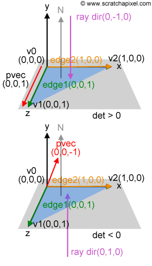
Note that when the ray and the normal of the triangle are facing each other (they go in opposite directions), the determinant is positive (greater than 0), as shown in the adjacent figure (top). On the other hand, when the ray hits the triangle from "behind" (the ray and the normal points in the same direction), the determinant is negative (adjacent figure, bottom). The figure on the side illustrates these two possible cases. The numbers are simple enough that cross and dot products between vectors are straightforward to compute. The coordinates of edge2 are (1,0,0), and the cross product between the ray direction (0,-1,0) and edge2 gives pvec. Remember that the cross product of two vectors is provided by:

$$ \begin{array}{l} x = v1.y v2.z - v1.z v2.y\\ y = v1.z v2.x - v1.x v2.z\\ z = v1.x v2.y - v1.y v2.x \end{array} $$

Thus:

$$ \begin{array}{l} pvec.z &=& dir.x * edge.y - dir.y * edge.x \\ &=& 0*0 -(-1 * 1) = 1, \end{array} $$

and pvec = (0,0,1). The dot product between this vector and edge1 (the determinant) is positive. When the ray has a direction (0,1,0), we get:

$$pvec.z = 0*0 - (1 * 1) = -1,$$

and pvec = (0,0,-1). The determinant is, in this case, negative.

In the original implementation of the algorithm (which you can find in the original paper, see reference below), the code can be either compiled to handle culling or ignored. When culling is active, rays intersecting triangles from behind will be discarded. This can easily be verified using the sign of the determinant. If culling is on and the determinant is lower than 0, then the ray doesn't intersect the triangle. However, when culling is off, we want to intersect triangles regardless of the normal orientation with resepct to the ray direction.

int intersect_triangle(...)
{
    ...
    det = DOT(edge1, pvec);
#ifdef CULLING        /* define CULLING if culling is desired */
    if (det < kEpsilon)
        return 0;
    ...
#else        /* the non-culling branch */
    if (det > -kEpsilon && det < kEpsilon)
        return 0;
    ...
#endif
}

The point we want to make here is that when culling is off and the determinant is negative, it becomes essential to "normalize \(u\)" by multiplying it by the inverse of the determinant. Because we later test if u is greater than 0 and lower than 1, when \(u\) is negative, but the determinant is also negative, then the sign of \(u\) when "normalized" (multiplied by invDet) is inverted (it becomes positive).

Source Code

The C++ implementation of the MT algorithm is straightforward (if you have an excellent vector library) and is also very compact, as you can see in this code snippet:

bool rayTriangleIntersect(
    const Vec3f &orig, const Vec3f &dir,
    const Vec3f &v0, const Vec3f &v1, const Vec3f &v2,
    float &t, float &u, float &v)
{
#ifdef MOLLER_TRUMBORE
    Vec3f v0v1 = v1 - v0;
    Vec3f v0v2 = v2 - v0;
    Vec3f pvec = dir.crossProduct(v0v2);
    float det = v0v1.dotProduct(pvec);
#ifdef CULLING
    // if the determinant is negative, the triangle is 'back facing'
    // if the determinant is close to 0, the ray misses the triangle
    if (det < kEpsilon) return false;
#else
    // ray and triangle are parallel if det is close to 0
    if (fabs(det) < kEpsilon) return false;
#endif
    float invDet = 1 / det;

    Vec3f tvec = orig - v0;
    u = tvec.dotProduct(pvec) * invDet;
    if (u < 0 || u > 1) return false;

    Vec3f qvec = tvec.crossProduct(v0v1);
    v = dir.dotProduct(qvec) * invDet;
    if (v < 0 || u + v > 1) return false;
    
    t = v0v2.dotProduct(qvec) * invDet;
    
    return true;
#else
    ...
#endif
}

Compile with:

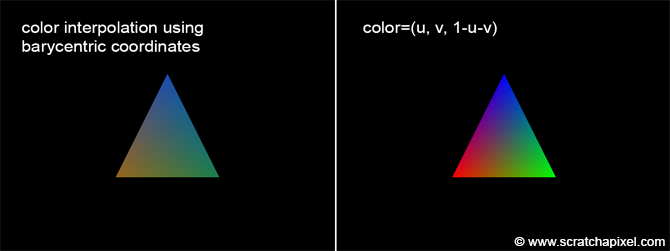
c++ -o raytri raytri.cpp -O3 -std=c++11 -DMOLLER_TRUMBORE

Important note regarding the MT algorithm implementation: If you compile the code provided with this lesson, you might notice that the image produced when the MT algorithm is used is not the same as the image of the triangle displayed above. This can be confusing. That's because the image of the triangle shown above was rendered using the geometry solution. Not the MT algorithm. The image below shows what the two algorithms output. On the left is the Möller–Trumbore solution. On the right is the geometric solution.

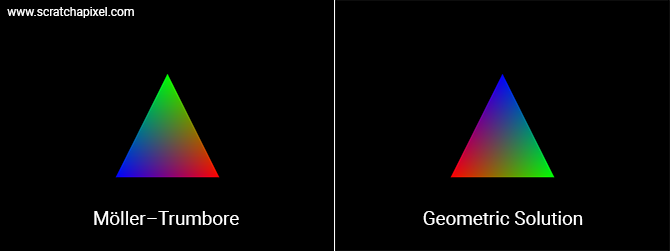
Why are they different? Mathematically they are not. It's just that the two algorithms are not calculating u, v, and w in the same order. The coordinate u in the geometric solution is equal to w in the MT solution, etc., and u in the first solution is numerically similar to w in the second. So don't worry. It's not because they produce a different image that one or the other is incorrect. They are both correct. You'll need to potentially swap the coordinates when using them for texturing and shading.

Notes

One way of accelerating the ray triangle is to store the constants A, B, C, and D of the plane equation with the triangle's vertices (we precompute them once the mesh is loaded and store them in memory). However, storing variables in memory and accessing them can be more expansive than the time required to compute them on the fly. Therefore this is not necessarily proven to be a reliable optimization.

One way of accelerating the algorithm is to reduce the ray-triangle intersection to two dimensions. To do so, we determine the dominant axis of the triangle's normal and use this information to select the two coordinates we use for the projection. This technique is described in "Ray-Polygon Intersection. An Efficient Ray-Polygon Intersection" (see references section below).

Algorithms to ray-trace quads already exist.

Our code uses single precision floating numbers, which are generally enough, but the ray-triangle intersection test may suffer from precision errors in some conditions. For example, the intersection point might not lie on the triangle plane and be either slightly above or below the triangle's surface. We will learn more about this in the lesson on shading.

Many of these topics are or will be addressed in the advanced section.

Exercises

• Add the camera transformation back to the source code of the main program.

• Compute more than one triangle with proper visibility using the trace() function we used in the previous lesson.

• Render a triangle from the back and test the culling branch of the code.

References

Fast, Minimum Storage Ray/Triangle Intersection. Möller & Trumbore. Journal of Graphics Tools, 1997.

Ray-Polygon Intersection. An Efficient Ray-Polygon Intersection. Didier Badouel from Graphics Gems I. 1990