Geometry

Creating an Orientation Matrix or Local Coordinate System

Reading time: 5 mins.

Constructing a Local Coordinate System from a Normal Vector

Throughout this chapter, we'll apply our understanding of coordinate systems to craft a local coordinate system (or frame) based around a vector, which can often be a normal. This method is frequently utilized within the rendering process to transition points and vectors from one coordinate system to another, positioning the normal at a given point as one axis of this local frame. This axis is typically aligned with the up vector, while the tangent and bi-tangent at that point establish the remaining orthogonal axes.

**Figure 1:** The tangent (T) and bi-tangent (B) reside in the tangent plane at point P. A cross product between T and B yields the surface normal N. These three vectors—T, B, and N—are orthogonal to each other, forming a Cartesian coordinate system.

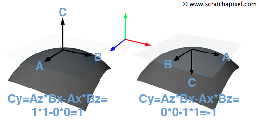
To form such a local frame accurately, one should employ the surface's normal, tangent, and bi-tangent at point P. These vectors lie within the plane tangent to P on the surface and must be orthogonal and normalized. In lessons on ray-geometry intersection calculations, the discussion will extend to computing derivatives at the intersection point—referred to as dPdu and dPdv. These derivatives provide a technical means of defining the tangent and bi-tangent at P. The normal at P is typically derived from the cross product of dPdu and dPdv. Attention must be paid to these vectors' orientations to ensure the cross-product results in a vector that extends outward from the surface, not inward. Knowing the directional orientation of these vectors allows for the application of the right-hand rule to ascertain the proper order for the cross product, ensuring the normal points away from the surface (refer to chapter 3 Math Operations on Points and Vectors for more).

**Figure 2:** Left, the cross product of A and B yields vector C, pointing away from the surface. Right, the cross product of B and A results in a vector pointing inward. The direction of the resultant vector can be determined using the right-hand rule.

Designating the normal N as the up vector, the tangent as the right vector, and the bi-tangent as the forward vector, these vectors can be arranged as rows in a [4x4] matrix as follows:

$$ \begin{bmatrix} T_x&T_y&T_z&0\\ N_x&N_y&N_z&0\\ B_x&B_y&B_z&0\\ 0&0&0&1 \end{bmatrix} $$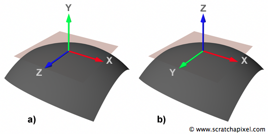

**Figure 3:** The arrangement of axis coordinates as rows in the orientation matrix hinges on the adopted convention. While the y-axis is typically the up vector, shading often treats the z-axis as such. Assuming a right-hand coordinate system, the z-axis in figure (a) should represent the tangent, with the x-axis as the bi-tangent. In figure (b), the y-axis would serve as the tangent, with the x-axis as the bi-tangent. Employing the right-hand mnemonic technique—index finger along the tangent and middle finger along the bi-tangent—helps determine the normal's direction.

When integrating this matrix within your code, it's crucial to be mindful of the specific context in which it's being used. For instance, certain portions of the code, particularly those related to shading, might adopt a different convention where the z-axis is treated as the up vector. This approach is often detailed in discussions on Spherical Coordinates, necessitating a reorganization of the matrix rows as follows to align with this shading-oriented convention:

$$ \begin{bmatrix} T_x&T_y&T_z&0\\ B_x&B_y&B_z&0\\ N_x&N_y&N_z&0\\ 0&0&0&1 \end{bmatrix} $$

This adjustment positions the normal vector's coordinates on the matrix's third row, adhering to the shading-centric convention of aligning the surface normal with the z-axis. While this alignment might not be immediately intuitive, it is a widely accepted standard within the shading domain, compelling us to adopt it for consistency's sake. As depicted in Figure 4, this convention contrasts with the world coordinate system, where the y-vector typically represents the up vector, by designating the z-vector as the up vector within the local coordinate system.

It's important to note that if your work involves a column-major order convention—contrary to Scratchapixel's row-major order—the vectors must be represented as columns rather than rows. This means that for a z-vector serving as the up vector, the coordinates of T would populate the first column, B's coordinates the second, and N's coordinates the third.

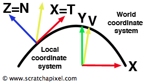
**Figure 4:** Expressing vector $V$ within a local coordinate framework, constructed from a surface point's normal $N$ and tangent $T$, simplifies by calculating the bitangent $B$ and utilizing these vectors to form a matrix. This matrix facilitates the transformation of $V$ from world space to a space defined by $N$, $T$, and $B$, a process particularly advantageous for shading. Note that $V$'s direction remains constant, though its coordinate representation shifts between the coordinate systems.

What purpose does this matrix serve? By applying it to a vector—$v$, for example, situated in world space—this matrix transitions $v$ into $v_M$, with its coordinates now defined relative to the locally constructed coordinate system anchored by $N$, $T$, and $B$. The absence of a translation component in this matrix's fourth row underscores its designation as an orientation matrix, aimed exclusively at vector manipulation. This feature proves invaluable in shading applications, where vector orientation in relation to the surface normal—typically aligned with the y- or z-axis by convention—greatly influences the computational process determining an object's color at the ray intersection point, as illustrated in Figure 4. This shading methodology will be explored comprehensively in the forthcoming lesson on Shading.

Affine Space: Certain rendering platforms, like Embree from Intel, favor an affine space representation for matrices and transformations. This approach delineates a Cartesian coordinate system through a specific space location (denoted as O) and three directional axes (Vx, Vy, Vz).