Geometry

How Does Matrix Work: Part 1

Reading time: 18 mins.

Understanding Conventions: A Cautionary Note

It might come as a surprise that the information presented here may not align perfectly with what you've encountered in other resources, whether books or online materials. While the core information remains consistent, you might notice variations in the order or sign of matrix coefficients. This discrepancy arises from the different conventions adopted by various authors or software. We encourage you to focus on the logic and principles outlined in this lesson, setting aside discrepancies with other sources for now. The following chapter will delve deeper into how these varying conventions influence both the theoretical presentation and practical implementation of matrices in programming.

To build on this, by the conclusion of this two-part series on the workings of matrices, we will offer a summary as clear and definitive as possible regarding the diverse conventions you may encounter across textbooks, resources, or source code. We will highlight sources of confusion that typically emerge, not just from the way mathematical equations involving matrices are written on paper but also from their actual implementation from a programming standpoint. Specifically, we will examine the nuances of row- versus column-major orderings, the implications of pre- and post-multiplication, and the interaction of matrices with related topics such as right versus left-hand coordinate systems. Don't worry if you don't know what these concepts are. We will explain them now.

Point-Matrix Multiplication Explored

This lesson aims to synthesize our understanding of points, vectors, matrices, and coordinate systems, paving the way for a comprehensive grasp of how matrices function. Building on the previous chapter's discussion on matrix compatibility for multiplication—specifically, that matrices of sizes m x p and p x n can be multiplied—we highlighted that in computer graphics, we predominantly work with 4x4 matrices.

Considering that a point or vector can be represented as a sequence of three numbers, they can also be conceptualized as 1x3 matrices. Here’s an illustration of a point expressed in matrix form:

$$P = [x y z].$$

By representing points and vectors as [1x3] matrices, we unlock the possibility of matrix multiplication. Keeping in mind that a m x p matrix can be multiplied by a p x n matrix to result in a m x n matrix, if we treat the first matrix as a point (thus, m = 1 and p = 3), it follows that the second matrix must take the form 3 x n, where n is any number greater than 1. Consequently, a [1x3] matrix can be multiplied by matrices of various forms, such as [3x1], [3x2], [3x3], [3x4], etc. Consider the multiplication of a [1x3] and a [3x4] matrix as an example:

$$ \begin{bmatrix}x & y & z\end{bmatrix} * \begin{bmatrix} c_{00}&c_{01}&{c_{02}}&c_{03}\\ c_{10}&c_{11}&{c_{12}}&c_{13}\\ c_{20}&c_{21}&{c_{22}}&c_{23}\\ \end{bmatrix} $$

To fully grasp the implications, we must bear in mind two key points. Firstly, multiplying a point by a matrix effectively transforms that point to a new location, implying the result must also be a point. Utilizing matrices for point transformation necessitates that the outcome of such multiplication yields another point, ideally represented as a 1x3 matrix. Consequently, to achieve a result that is also a point, the multiplying matrix must be a 3x3 matrix. The product of a 1x3 and a 3x3 matrix, as expected, yields a 1x3 matrix—a transformed point. Here’s how this multiplication manifests:

$$ \begin{bmatrix}x & y & z\end{bmatrix} * \begin{bmatrix} c_{00}&c_{01}&{c_{02}}\\ c_{10}&c_{11}&{c_{12}}\\ c_{20}&c_{21}&{c_{22}}\\ \end{bmatrix} $$

In computer graphics (CG), while 4x4 matrices are often the standard, there are instances where we initially work with 3x3 matrices. The reasons for favoring 4x4 matrices will be clarified shortly, but for the moment, let's concentrate on understanding 3x3 matrices. As we wrap up this portion of the chapter, we'll demonstrate through pseudocode how to multiply a point $P$ (or a vector represented in matrix form) by a 3x3 matrix to yield a transformed point $P_T$. Should you need to revisit the basics of matrix multiplication, please refer back to the previous chapter. The process involves multiplying each element of a row in the first matrix by the corresponding element of a column in the second matrix, then summing these products to compute each element of the resultant matrix. The pseudocode below illustrates this process, and we'll discuss the 4x4 matrix case later on:

// For the x-component, combine row 1 elements with column 1 elements
Ptransformed.x = P.x * c00 + P.y * c10 + P.z * c20
// For the y-component, combine row 1 elements with column 2 elements
Ptransformed.y = P.x * c01 + P.y * c11 + P.z * c21
// For the z-component, combine row 1 elements with column 3 elements
Ptransformed.z = P.x * c02 + P.y * c12 + P.z * c22

Understanding the Identity Matrix

The identity matrix, also known as the unit matrix, is a special type of square matrix. Its off-diagonal elements are all zeros, while the diagonal elements are all ones:

$$ \begin{bmatrix} \color{red}{1} & 0 & 0 \\ 0 & \color{red}{1} & 0 \\ 0 & 0 & \color{red}{1} \end{bmatrix} $$

Multiplying a point $P$ by the identity matrix yields $P$ itself. This property becomes evident when we integrate the identity matrix coefficients into our point-matrix multiplication pseudocode, illustrating the identity matrix's role in preserving the original point:

// Multiplying P by the identity matrix results in P
Ptransformed.x = P.x * 1 + P.y * 0 + P.z * 0 = P.x
Ptransformed.y = P.x * 0 + P.y * 1 + P.z * 0 = P.y
Ptransformed.z = P.x * 0 + P.y * 0 + P.z * 1 = P.z

Exploring the Scaling Matrix

When examining the process of point-matrix multiplication, it's apparent that the coordinates of point $P$ are individually multiplied by specific coefficients along the matrix's diagonal: $R_{00}$ for the x-coordinate, $R_{11}$ for the y-coordinate, and $R_{22}$ for the z-coordinate. Setting these diagonal coefficients to 1, with all other matrix elements at 0, yields the identity matrix, effectively leaving $P$ unchanged. However, altering these diagonal values to something other than 1 scales the point's coordinates either up or down, depending on whether these values are greater or smaller than 1. This observation ties back to our discussion on coordinate systems, where we noted that scaling a point's coordinates is achieved by multiplying them by some scalar values. Consequently, the scaling matrix is expressed as:

$$ \begin{bmatrix} \color{red}{S_X} & 0 & 0 \\ 0 & \color{red}{S_Y} & 0 \\ 0 & 0 & \color{red}{S_Z} \end{bmatrix} $$

Here, $S_X$, $S_Y$, and $S_Z$ represent the scaling factors for each respective axis.

// Applying the scaling matrix to P
Ptransformed.x = P.x * Sx + P.y * 0  + P.z * 0  = P.x * Sx
Ptransformed.y = P.x * 0  + P.y * Sy + P.z * 0  = P.y * Sy
Ptransformed.z = P.x * 0  + P.y * 0  + P.z * Sz = P.z * Sz

For instance, consider a point $P$ with the coordinates (1, 2, 3). Applying a scaling matrix with $Sx = 1$, $Sy = 2$, and $Sz = 3$ transforms $P$ into a new point with coordinates (1, 4, 9), effectively scaling each coordinate by the specified factors.

It's also worth noting that using negative values for any of the scaling coefficients will invert the corresponding coordinate across that axis, akin to reflecting the point across the axis. This feature allows for mirror transformations in addition to scaling.

Understanding the Rotation Matrix

This section delves into constructing a matrix that rotates a point or vector around an axis within the Cartesian coordinate system, utilizing trigonometric functions for the operation.

**Figure 1:** a 90 degrees counterclockwise rotation.

Consider a point $P$ in a three-dimensional space, positioned at (1, 0, 0). Temporarily disregarding the z-axis and focusing on the xy plane, our goal is to rotate $P$ to a new position $P_T$ with coordinates (0, 1, 0). This rotation can be visualized in Figure 1, where $P$ is rotated 90 degrees counterclockwise around the z-axis to reach $P_T$. Suppose we have a rotation matrix $R$. Multiplying $P$ by $R$ results in the transformation of $P$ to $P_T$. To understand this transformation through matrix multiplication, let's break down the calculation for each coordinate of the transformed point:

$$ \begin{array}{l} P_T.x = P.x * R_{00} + P.y * R_{10} + P.z * R_{20}\\ P_T.y = P.x * R_{01} + P.y * R_{11} + P.z * R_{21}\\ P_T.z = P.x * R_{02} + P.y * R_{12} + P.z * R_{22}\\ \end{array} $$

**Figure 2:** a 45 degrees counterclockwise rotation.

For our purposes, $P_T.z$ is of lesser concern since it pertains to the z-coordinate of $P_T$. Our focus lies on $P_T.x$ and $P_T.y$, which denote the x and y coordinates of $P_T$, respectively. Observing the transition from $P$ to $P_T$, the x-coordinate changes from 1 to 0, indicating that $R_{00}$ must be 0. Given that both $P.y$ and $P.z$ are zero, the exact values of $R_{10}$ and $R_{20}$ are momentarily irrelevant. Transitioning from $P$ to $P_T$, the y-coordinate increases from 0 to 1. Considering $P.x$ is 1 and its other coordinates are null, it implies $R_{01}$ must be 1. Summarizing, we've deduced $R_{00} = 0$ and $R_{01} = 1$. Let's document this and examine what $R$ looks like in comparison to the identity matrix:

$$ R_z= \begin{bmatrix} 0 & 1 & 0 \\ 1 & 0 & 0 \\ 0 & 0 & 1 \\ \end{bmatrix} $$

At this point, don't stress about the specific values of the coefficients—clarification is forthcoming. The key takeaway is that applying this rotation matrix to $P = (1, 0, 0)$ yields $P_T = (0, 1, 0)$, demonstrating the matrix's role in facilitating the rotation.

Continuing from the rotation matrix discussion, when applying the matrix $R$ to transform $P$ to $P_T$, the operation simplifies to:

$$ \begin{array}{l} P_T.x = P.x * 0 + P.y * 1 + P.z * 0 = 0\\ P_T.y = P.x * 1 + P.y * 0 + P.z * 0 = 1\\ P_T.z = P.x * 0 + P.y * 0 + P.z * 1 = 0\\ \end{array} $$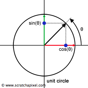

**Figure 3:** cosine and sine can be used to determine the coordinate of a point on the x- and y-axis of the unit circle.

Knowledge of trigonometric functions will now turn out to be handy. As you know, for a point on the unit circle, its x and y coordinates correlate with the cosine and sine of the angle $\theta$, respectively, as illustrated in Figure 3:

$$ \begin{array}{l} x = \cos(\theta) = 0\\ y = \sin(\theta) = 1\\ \text{given } {\theta = {\pi \over 2}}\\ \end{array} $$

At $\theta$ = 0, we find x = 1 and y = 0. At $\theta$ = 90 degrees (or $\pi \over 2$), x becomes 0 and y turns to 1. Interestingly, these values correspond to $R_{00}$/$R_{11}$ and $R_{01}$/$R_{10}$, allowing us to redefine the rotation matrix $R$ for a $\theta$ of 90 degrees ($\pi \over 2$) as:

$$R_z(\theta)= \begin{bmatrix} \cos(\theta) & \sin(\theta) & 0 \\ \sin(\theta) & \cos(\theta) & 0 \\ 0 & 0 & 1 \\ \end{bmatrix} = \begin{bmatrix} 0 & 1 & 0 \\ 1 & 0 & 0 \\ 0 & 0 & 1 \\ \end{bmatrix} \text{ with } {\theta = {\pi \over 2}} $$

Applying a 45-degree rotation ($\pi \over 4$) using $R$ to $P$, $P_T$ achieves coordinates (0.7071, 0.7071), confirming the correctness of this approach (Figure 2). Hence, the rotation matrix for the z-axis becomes:

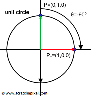
$$ R_z(\theta)= \begin{bmatrix} \cos(\theta) & \sin(\theta) & 0 \\ \sin(\theta) & \cos(\theta) & 0 \\ 0 & 0 & 1 \\ \end{bmatrix} $$

However, considering a rotation of 90 degrees clockwise (Figure 4), we examine whether $R$ accurately performs this transformation from $P$ = (0, 1, 0) to $P_T$ = (1, 0, 0):

$$ R_z= \begin{bmatrix} \cos(-{\pi \over 2}) & \sin(-{\pi \over 2}) & 0 \\ \sin(-{\pi \over 2}) & \cos(-{\pi \over 2}) & 0 \\ 0 & 0 & 1 \\ \end{bmatrix}= \begin{bmatrix} 0 & -1 & 0 \\ -1 & 0 & 0 \\ 0 & 0 & 1 \\ \end{bmatrix} $$ $$ \begin{array}{lll} P_T.x = &0 * R_{00} &+& 1 * R_{10} &+& P.z * R_{20} &= \\ &0*0 &+& 1*-1 &+& 0*0&=-1\\ P_T.y = &0 * R_{01} &+& 1 * R_{11} &+& P.z * R_{21} &= \\ &0*-1 &+& 1*0 &+& 0*0&= 0\\ P_T.z = &0 * R_{02} &+& 1 * R_{12} &+& P.z * R_{22} &= \\ &0*0 &+& 1*0 &+& 0*1&= 0\\ \end{array} $$

The direct application yields (-1, 0, 0) instead of (1, 0, 0), suggesting a need for adjustment. Correcting this, the proper rotation matrix for a clockwise rotation becomes:

$$ R_z= \begin{bmatrix} \cos(-{\pi \over 2}) & \sin(-{\pi \over 2}) & 0 \\ -\sin(-{\pi \over 2}) & \cos(-{\pi \over 2}) & 0 \\ 0 & 0 & 1 \\ \end{bmatrix}= \begin{bmatrix} 0 & -1 & 0 \\ 1 & 0 & 0 \\ 0 & 0 & 1 \\ \end{bmatrix} $$ $$ \begin{array}{lll} P_T.x = &0 * R_{00} &+& 1 * R_{10} &+& P.z * R_{20} &= \\ &0*0 &+& 1*1 &+& 0*0&=1\\ P_T.y = &0 * R_{01} &+& 1 * R_{11} &+& P.z * R_{21} &= \\ &0*-1 &+& 1*0 &+& 0*0&= 0\\ P_T.z = &0 * R_{02} &+& 1 * R_{12} &+& P.z * R_{22} &= \\ &0*0 &+& 1*0 &+& 0*1&= 0\\ \end{array} $$

This yields the correct transformed coordinates of $P_T$ as (1, 0, 0), illustrating the matrix's ability to accurately rotate points around the z-axis without altering the z-coordinate.

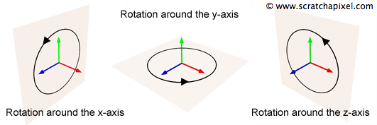
**Figure 4:** a 90 degrees clockwise rotation.

The matrices for rotations around the x and y axes can be derived similarly, with $R_x$ affecting rotations in the yz plane and $R_y$ in the xz plane. Here are the matrices for rotations around the x and y axes (with $R_z$ for completness):

$$ R_x(\theta)= \begin{bmatrix} 1 & 0 & 0 \\ 0 & \cos(\theta) & \sin(\theta) \\ 0 & -\sin(\theta) & \cos(\theta) \\ \end{bmatrix} $$ $$ R_y(\theta)= \begin{bmatrix} \cos(\theta) & 0 & -\sin(\theta) \\ 0 & 1 & 0 \\ \sin(\theta) & 0 & \cos(\theta) \\ \end{bmatrix} $$ $$ R_z(\theta)= \begin{bmatrix} \cos(\theta) & \sin(\theta) & 0\\ -\sin(\theta) & \cos(\theta) & 0\\ 0 & 0 & 1 \\ \end{bmatrix} $$

To calculate the transformed point's coordinates, you multiply the point's coordinates by the coefficients in each column of these matrices, ensuring a consistent approach to point transformation across different axes of rotation.

If you've been comparing the rotation matrices provided here with those on Wikipedia's page about rotation matrices and noticed discrepancies, you're not alone. The matrices listed on Wikipedia appear as follows:

$$ \begin{alignat}{1} R_x(\theta) &= \begin{bmatrix} 1 & 0 & 0 \\ 0 & \cos \theta & -\sin \theta \\[3pt] 0 & \sin \theta & \cos \theta \\[3pt] \end{bmatrix} \\[6pt] R_y(\theta) &= \begin{bmatrix} \cos \theta & 0 & \sin \theta \\[3pt] 0 & 1 & 0 \\[3pt] -\sin \theta & 0 & \cos \theta \\ \end{bmatrix} \\[6pt] R_z(\theta) &= \begin{bmatrix} \cos \theta & -\sin \theta & 0 \\[3pt] \sin \theta & \cos \theta & 0 \\[3pt] 0 & 0 & 1 \\ \end{bmatrix} \end{alignat} $$

Indeed, these appear quite different from the ones we've discussed. However, this discrepancy underscores the critical importance of understanding the conventions underpinning these matrices. To accurately interpret a matrix, you need to know:

Whether the coordinate system is left-handed or right-handed.
Whether the matrices are used in column-major or row-major order.

The Wikipedia article specifies that the matrices are based on a right-hand coordinate system (similar to our usage on Scratchapixel) but employs the column-major convention. On the other hand, we use the row-major order convention. This difference means that to align Wikipedia's matrices with ours, one must transpose them. A matrix transpose—detailed in our Matrix Operations chapter—leaves diagonal coefficients unchanged while flipping the others across the diagonal. For example, a coefficient at position m[0][1] moves to m[1][0] after transposition. Applying this transposition to Wikipedia's matrices yields matrices identical to ours:

$$ \begin{alignat}{1} R_x(\theta) &= \begin{bmatrix} 1 & 0 & 0 \\ 0 & \cos \theta & \sin \theta \\[3pt] 0 & -\sin \theta & \cos \theta \\[3pt] \end{bmatrix} \\[6pt] R_y(\theta) &= \begin{bmatrix} \cos \theta & 0 & -\sin \theta \\[3pt] 0 & 1 & 0 \\[3pt] \sin \theta & 0 & \cos \theta \\ \end{bmatrix} \\[6pt] R_z(\theta) &= \begin{bmatrix} \cos \theta & \sin \theta & 0 \\[3pt] -\sin \theta & \cos \theta & 0 \\[3pt] 0 & 0 & 1 \\ \end{bmatrix} \end{alignat} $$

This exemplifies the importance of recognizing the conventions used, particularly regarding coordinate systems (left or right-handed) and matrix order (row-major or column-major). The choice of convention in your work is flexible, provided it's communicated clearly to others who may use your code. On Scratchapixel, we consistently use right-hand coordinate systems and row-major order matrices, chosen for historical reasons, although we acknowledge the benefit of a universal standard. For instance, Maya, a 3D software, uses a right-hand coordinate system but adopts a column-major order for matrices, while Pixar's rendering engine, PRMAN, prefers row-major order matrices by default.

Navigating the realm of CGI programming, one quickly realizes that the concepts of "right" and "wrong" are often not as black-and-white as they seem. If you're feeling bewildered by encountering different sets of equations in various resources, it's a natural part of the learning curve. Perhaps you've started with a book presenting one methodology, only to find contrasting approaches elsewhere, like on Scratchapixel. It's important to acknowledge that Scratchapixel strives to clarify the reasons behind these differences, emphasizing the significance of understanding the conventions in play.

This attention to the nuances of mathematical conventions, whether it involves coordinate systems or matrix order, is crucial. While it might be a source of frustration and confusion initially, recognizing and adapting to these discrepancies is an integral skill in the CGI field. As you progress in your career, you'll likely encounter these variations almost daily in your work. Thus, rather than viewing them as obstacles, consider them as opportunities to deepen your understanding and flexibility in navigating the complex landscape of computer graphics and interactive programming.

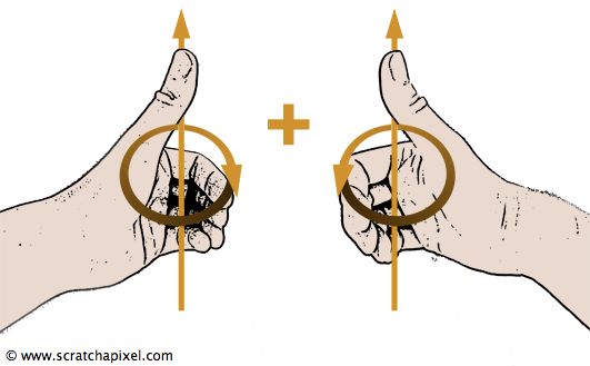
**Figure 5:** rotations around the x-, y-, and z-axis. The arrow indicates the rotation direction for positive angles.

**Figure 6:** Using the left-hand coordinate system (left), curl your fingers around the axis of rotation to determine the direction of positive rotations. For the right-hand coordinate system, repeat with your right hand.

The mnemonic technique mentioned earlier helps easily determine the direction of rotation for positive angles, especially when using a right-hand coordinate system. Curling your fingers around the axis of rotation, as shown in Figure 6, intuitively indicates the direction of positive rotations:

right-hand system: counter-clockwise.
left-hand system: clockwise.

Synthesizing Rotation Matrices

From the insights gained in the preceding chapter, we understand that the act of multiplying matrices effectively amalgamates their transformation effects. With the knowledge of how to enact rotations around each cardinal axis, we are now equipped to craft more intricate rotational dynamics by combining $R_x$, $R_y$, and $R_z$ matrices. For instance, if the aim is to first rotate a point around the x-axis followed by the y-axis, this can be achieved by creating two matrices from $R_x$ and $R_y$ and merging them through matrix multiplication ($R_x * R_y$) to forge a composite $R_{XY}$ matrix that embodies both rotations:

$$R_{XY} = R_X * R_Y$$

It's crucial to note that the sequence of rotations significantly impacts the outcome. Rotating a point initially around the x-axis and subsequently around the y-axis typically yields a distinct result compared to performing these rotations in the reverse order. This principle of rotation order is a fundamental aspect in many 3D modeling and animation software like Maya, 3DSMax, Softimage, and Houdini, where users can specify the rotation sequence, such as xyz, among other configurations.

Introducing the Translation Matrix

To facilitate point translations via point-matrix multiplication, the adoption of [4x4] matrices becomes indispensable. Given that our current discussion is constrained to [3x3] matrices, the intricacies of utilizing matrices for translations will be expounded upon in the Transforming Points and Vectors chapter.

Rotations Around an Arbitrary Axis

While it is entirely feasible to devise a routine that rotates a point or vector around any given axis, such an endeavor is deemed beyond the scope of constructing a rudimentary ray tracer. The exploration of this topic is slated for future updates to this lesson series, following a thorough examination of foundational concepts.