How Does Matrix Work: Part 2
Reading time: 11 mins.Understanding the Link Between Matrices and the Cartesian Coordinate System
Consider a scenario where you have a point \(P_x\) with coordinates (1, 0, 0), and you wish to rotate it around the z-axis by 10 degrees in a clockwise direction. How would the coordinates of this point change? Using rotation matrices and basic trigonometry, we can determine the new coordinates. The x-coordinate of the newly rotated point \(P_x\) can be calculated using \(\cos(-10^\circ)\), while the y-coordinate is obtained using \(\sin(-10^\circ)\) (noting that trigonometric functions in C++ require angles to be in radians). Similarly, if we rotate a point \(P_y\) with coordinates (0, 1, 0) by the same angle, the resulting x-coordinate will be \(-\sin(-10^\circ)\), and the y-coordinate will be \(\cos(-10^\circ)\).
It’s interesting to note that the trigonometric functions used to calculate the new coordinates of \(P_x\) are reflected in the first row of the rotation matrix \(R_Z\), which is used for rotating points around the z-axis. A similar pattern appears in the matrix's second row, corresponding to the trigonometric calculations for the rotated \(P_y\) coordinates:
$$ \begin{array}{ll} P_x^x = \cos(\theta) & P_x^y = \sin(\theta) \\ P_y^x = -\sin(\theta) & P_y^y = \cos(\theta) \end{array} $$As we rotate the axes around the z-axis, the computation of new coordinates for \(P_x\) aligns with the matrix's first row, while \(P_y\)’s coordinates align with the second row. If this process is applied to a point \(P_z\) using the rotation matrices \(R_X\) or \(R_Y\), \(P_z\)’s new coordinates would come from the third row of the chosen matrix, depending on which axis is used for rotation.
The essence of matrices is that each row represents an axis (or basis) of a coordinate system. This understanding is crucial, as it lays the foundation for learning how to create matrices that transform points and vectors between coordinate systems (change of basis). This is done by substituting the matrix rows with the coordinates of the new coordinate system's axes into which you want to transform your vectors or points:
$$ \begin{bmatrix} \color{red}{c_{00}} & \color{red}{c_{01}} & \color{red}{c_{02}} \\ \color{green}{c_{10}} & \color{green}{c_{11}} & \color{green}{c_{12}} \\ \color{blue}{c_{20}} & \color{blue}{c_{21}} & \color{blue}{c_{22}} \end{bmatrix} \begin{array}{l} \rightarrow \quad \color{red} {x\text{-axis}} \\ \rightarrow \quad \color{green} {y\text{-axis}} \\ \rightarrow \quad \color{blue} {z\text{-axis}} \end{array} $$This technique, a fundamental concept in computer graphics, will be explored further in later chapters. The mystery around matrices fades when you realize that they store the coordinates of a coordinate system, with each matrix row representing one of the system's axes. This is sometimes referred to as an orientation matrix.
The discussion above pertains to matrices in row-major order, where each row of the matrix corresponds to an axis of the Cartesian coordinate system. It is important to highlight that things are different when working with column-major order matrices. In column-major matrices, each column, rather than each row, represents one of the Cartesian coordinate system's axes (x, y, and z). Therefore, when using column-major matrices for transformations, each column of the matrix represents one of the coordinate system's axes or basis vectors, not the rows.
In 4x4 matrices, the translation components are specifically positioned, and this positioning depends on the matrix’s order:
-
Row-major order matrices: The translation values are located in the matrix’s fourth row, at
m[3][0],m[3][1], andm[3][2]for the x, y, and z translations, respectively. This placement integrates translation with rotation and scaling operations within a single matrix, streamlining transformations in three-dimensional space. -
Column-major order matrices: The translation values are placed in the fourth column.
Similar to other concepts I’ve explained or will explain in this lesson, some of the ideas I’m referring to haven’t been covered yet. For example, the concept of row-major vs. column-major matrices is something we’ll talk about later in the chapter Row Major vs. Column Major Vector and Matrices. When I initially wrote this lesson more than 10 years ago, likely around 2009, I didn’t pay much attention to these cross-dependencies. It’s only today, while re-reading the lesson years later, that I realized this. Ideally, I would restructure this lesson, but given limited time and resources, please bear with me for now until I find the time to do so.
Regarding row-major vs. column-major matrices (and vectors), and until we get to the chapter dedicated to that, let’s briefly summarize: these are just two different ways of writing matrices. In row-major order, the coefficients are written as rows, where each row represents a direction of the Cartesian coordinate system. In column-major order, the same numbers or coefficients are written as columns. There’s no difference in the actual matrix; it’s just a different way of arranging the coefficients, either horizontally or vertically. Different people prefer one convention over the other, often based on their background (mathematics, physics, computer graphics programming) or the system they were first introduced to.
The way you write matrices or vectors—either horizontally or vertically—doesn't change the outcome of a calculation. Transforming a point or vector with a matrix will yield the same Cartesian coordinates regardless of the convention used. What changes is how matrix-vector multiplication is written on paper. With row-major matrices, vector-matrix multiplication is written as \( P \times M \), whereas in column-major notation, it’s written as \( M \times P \). These details are explained further in the chapter Row Major vs. Column Major Vector and Matrices.
Now that you have a basic understanding of the differences between these two conventions, the key point is that the location of the coefficients is important for understanding how transformations are applied and interpreted. If you know that a paper or code assumes matrices are in row-major order, then you can be sure that each row represents one of the Cartesian coordinate system’s basis vectors. If the convention is column-major, then each column represents one of these basis vectors. This highlights the fact that understanding the convention being used before diving into any material is absolutely necessary.
I realize we haven’t yet discussed why we use 4x4 matrices instead of 3x3 matrices, which we’ve only considered so far for studying point rotation and scaling. Mentioning them here might feel a bit confusing, and I’m aware of that. However, don’t worry—this will be covered in detail in the next chapter. For now, let’s just note that, as mentioned earlier, the fourth row in a [4x4] matrix is used to store the translation we want to apply to our point. In a row-major matrix, these coefficients are stored in the fourth row; in a column-major matrix, they are stored in the fourth column.
Additionally, you might wonder why we don’t use a 4x3 matrix. After all, we need four rows but only three columns to store the x, y, and z coordinates of the Cartesian axes and the translation values. If you’re asking this question, it’s a great sign that you’ve understood the material so far. The reason we use [4x4] matrices (and not [4x3])—which also means the point should be represented as a [1x4] vector by the way—won’t be answered here, but rest assured, it will be explained later in the lesson.
To clarify this further, let’s consider another example. Let’s rotate an object in Maya by 45 degrees. Maya uses a right-handed coordinate system and row-major matrices. The resulting matrix for this rotation is:
$$ M = \begin{bmatrix} 0.707107 & 0.707107 & 0 & 0 \\ -0.707107 & 0.707107 & 0 & 0 \\ 0 & 0 & 1 & 0 \\ 0 & 0 & 0 & 1 \end{bmatrix} $$This is a 4x4 transformation matrix, where:
-
The first row is \([0.707107, 0.707107, 0, 0]\),
-
The second row is \([-0.707107, 0.707107, 0, 0]\),
-
The third row is \([0, 0, 1, 0]\),
-
The fourth row is \([0, 0, 0, 1]\).
In row-major matrices (such as in Maya), the rows represent the axes of the coordinate system.
-
The first row \([0.707107, 0.707107, 0]\) represents the transformed x-axis after the 45-degree rotation.
-
The second row \([-0.707107, 0.707107, 0]\) represents the transformed y-axis after the rotation.
-
The third row \([0, 0, 1]\) represents the z-axis, which remains unchanged because the rotation occurs in the X-Y plane.
This transformation matrix corresponds to a 45-degree rotation about the z-axis in a right-handed coordinate system (as used in Maya). The 0.707 values appear because:
$$\cos(45^\circ) = 0.707107 \quad \text{and} \quad \sin(45^\circ) = 0.707107$$Thus, the object is rotated counterclockwise by 45 degrees around the z-axis, and the new x and y axes are reflected in the first two rows of the matrix.
In row-major systems, the rows of the matrix directly represent the basis vectors or coordinate axes in the transformed space:
-
The first row represents the direction of the new x-axis in the 3D space after transformation.
-
The second row represents the direction of the new y-axis.
-
The third row represents the z-axis.
This means that after the 45-degree rotation, the x-axis points in the direction \([0.707107, 0.707107, 0]\), and the y-axis points in the direction \([-0.707107, 0.707107, 0]\), while the z-axis remains \([0, 0, 1]\).
Comparing this with column-major matrices (like those used in OpenGL or GLSL):
-
In row-major matrices (like Maya’s): Each row of the matrix represents an axis of the coordinate system.
-
In column-major matrices (like OpenGL’s): Each column represents an axis of the coordinate system.
So, in Maya, where matrices are stored in row-major order, the rows represent the transformed coordinate axes. This is why the first row holds the new x-axis, the second row holds the new y-axis, and so on.
Orthogonal Matrices and Their Role in Linear Algebra
Orthogonal matrices, a central topic discussed in this and the preceding chapter, are square matrices with real entries where both columns and rows consist of orthogonal unit vectors. These matrices, particularly rotation matrices or those derived from multiplying several rotation matrices, inherently represent the axes of a Cartesian coordinate system with unit length axes. This characteristic arises because their row elements are derived from sine and cosine functions, which calculate points on the unit circle, mirroring a Cartesian coordinate system initially aligned with the world coordinate system (where the identity matrix's rows signify the world coordinate system's axes) that has been rotated around a specific or arbitrary axis. A key attribute of orthogonal matrices, highly valuable in Computer Graphics, is their property where the transpose of an orthogonal matrix equals its inverse. Represented mathematically as \(Q^T=Q^{-1}\), it implies \(QQ^T=I\), with \(I\) being the identity matrix. Because of this property, it is easy to reverse transformations; you simply need to transpose the orthogonal matrix. You can find information on matrix transposition in the chapter on Matrix Operations.
Affine Transformations in Computer Graphics
The term affine transformations is often used in place of matrix transformations, providing a more accurate name for the types of transformations we’ve discussed so far. Affine transformations are special because they are linear and keep points, straight lines, and planes intact. Common transformations like translation, rotation, and shearing are examples of affine transformations, as are any combinations of these. This leads to the concept of projective transformations in computer graphics, which include perspective projection. Projective transformations can change how parallel lines appear, a topic that will be covered in more detail when we discuss perspective and orthographic projection matrices in the Foundations of 3D Rendering section.
The key takeaway here is that if you come across the term "affine transformation" in a text, you should know that it's just another name for a basic 4x4 matrix—nothing more, nothing less. It's not some fancy term hiding complicated mathematics or properties. And by "simple 4x4 matrix," I mean a matrix that doesn’t involve projection, like a perspective projection matrix.
Takeaways
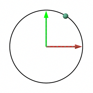
The last two chapters not only explain how to construct rotation matrices but also provide a conceptual framework for understanding matrices. Each row of a matrix (assuming a row-major ordered matrix) can be viewed as an axis within a Cartesian coordinate system, with the entire matrix representing the transformation (such as rotation, scale, or translation) applied to points when multiplied. This framework suggests that points defined in one coordinate system (A), and attached to a local coordinate system (B) or matrix, will retain their coordinates relative to B, even as B undergoes transformations. However, their coordinates relative to A will change, illustrating the effects of the transformation. This concept is visually depicted in Figure 6, which shows how a point's coordinates change relative to the world coordinate system while remaining constant relative to the coordinate system defined by the rotation matrix during rotation.
Key takeaways include the derivation of basic rotation matrices, the significance of matrix multiplication order, and the conceptualization of a matrix as a local Cartesian system (or orientation matrix). This understanding is further expanded upon in the chapter Creating an Orientation Matrix or Local Coordinate System, emphasizing the foundational role of matrices in graphical transformations.