Introduction to Shading

Diffuse and Lambertian Shading

Reading time: 22 mins.

Diffuse or Lambertian Shading

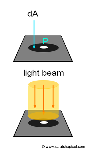
**Figure 1:** A light beam illuminating a small surface $dA$.

Diffuse objects are easy to simulate in CG. However, to understand how it works, we first need to learn about the way light interacts with surfaces. Technically, to understand this topic thoroughly, we should study radiometry first. To keep this introduction simple and intuitive, we will proceed without it. Simplifying the concept, when we shade a point in CG, we assume this point represents a very small surface, which we call a differential area. Don’t focus too much on the term "differential" here, and pay attention instead to the term "area." Rather than considering a theoretical point that has no physical meaning, we will be considering a very small area around the point, which we generally denote in CG as $dA$. Additionally, we consider the amount of light falling on the surface of this very small area around $P$. Light that falls at $P$ is not reduced to a single light ray, since we are not interested in a singular point, but the small region $dA$ around that point. Light that falls on this region is contained within a small volume perpendicular to $P$, as shown in the left illustration of the following figure.

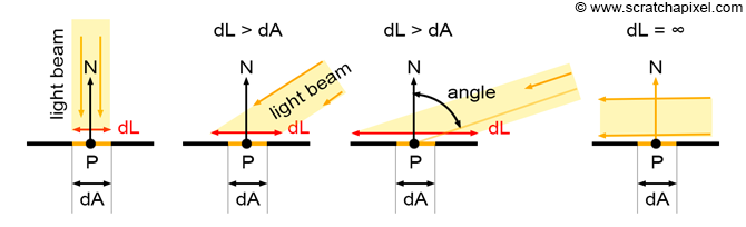
In other words, all light energy contained within this volume, which has the same cross-section as $dA$, falls on $dA$. If a constant flux of light energy travels through this volume as depicted in the left image of the above illustration, then one can assume that there's a constant amount of light energy striking the surface $dA$ at any given time. Another way of saying this is to imagine that 1000 photons strike the surface of $dA$ at any given time. These 1000 photons will interact with the object's surface: some will be absorbed, and some will be reflected almost simultaneously. A fraction of time later, 1000 new photons will strike the surface of $dA$ again. If the flux of photons is constant, then this process keeps repeating itself. Since the cone of light perpendicular to $dA$ has the same cross-section as $dA$, $dA$ is constantly bombarded by 1000 photons every fraction of time (which in CG we often refer to as $dt$, a concept similar to $dA$ but applied to time). An interesting occurrence happens when this cone of light is angled with regard to the normal at $P$. As you can see in the second and third illustrations of the above image, as the angle between the light beam and the normal at $P$ increases, the cross-section of the beam with the surface of the object becomes larger than $dA$. To put it differently, of the 1000 photons that used to strike $dA$, only a fraction of these photons arrive at $dA$ when the light beam makes an angle with the normal. That fraction (the number of photons received by $dA$ over the total number of photons contained in the beam) becomes smaller as the angle increases. When the light beam is perpendicular to the object's surface, no photons strike $dA$ at all.

To summarize:

When the light beam is perpendicular to $dA$, 100% of the photons within the small cone of light, whose cross-section is the same as $dA$, strike $dA$.
When the light beam makes an angle with the normal of the shaded point, then the cross-section of the beam with the surface becomes larger than $dA$. This means that the photons or light energy are distributed over a larger region than $dA$. Since we are only interested in the amount of light energy arriving over the region covered by $dA$, we can also say that fewer photons reach $dA$ as the angle of the light beam with the normal increases. The larger the angle, the fewer the photons. Thus, $dA$ keeps receiving less and less energy as the angle between the beam and the normal increases.
In the extreme case, when the beam is perpendicular to the normal at $P$, then photons do not fall on $dA$ at all. In this particular case, $dA$ does not receive any light energy at all.

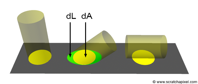
**Figure 2:** The cosine law. The amount of light incident on the surface depends on the cosine of the angle between the light incident direction and the surface normal. The differential area $dA$ receives more light energy when this angle is small.

From these observations, it becomes easier to understand that a surface element $dA$ receives a maximum of light energy when the beam is perpendicular to the surface, or in other words, when the surface normal $N$ and the light direction $L$ are parallel. However, when the light beam illuminates the surface from a certain angle, $dA$ receives less light energy than when the beam is perpendicular to the surface, which means that the surface itself will also reflect less light into the environment. We can naturally deduce from this that the surface will get darker. As mentioned earlier, as the angle between $N$ and $L$ increases, $dA$ is hit by fewer and fewer photons. In practical terms, this means that the surface gets darker and darker as the angle between the two vectors increases. Ultimately, when $N$ and $L$ are perpendicular, $dA$ receives no light at all and is therefore black (since it receives no light, it reflects none either). More generally, we can say that the brightness is proportional to the ratio $dA$ over $dL$. Since $dL$, the oblique cross-section of the light beam, becomes larger as the angle between the two vectors increases, this ratio decreases as the angle increases.

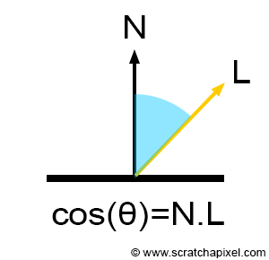
This principle is one of the most basic and well-known phenomena in CG. It is known under the name of Lambert's Cosine Law. The amount of light that a surface receives is directly proportional to the angle between the surface normal $N$ and the light direction $L$. This angle can be defined mathematically as:

$$\cos\theta = N \cdot L$$

Hence the term cosine is in the law's name. The cosine of the angle $\theta$ (the Greek letter theta) is defined as the dot product of the vector $N$ and $L$. If there is one thing you should remember from this lesson, it should probably be this fundamental law. Of course, the amount of light a surface reflects, and thus how bright it appears, depends directly on the amount of light it receives. Thus we can somehow write that the final color of a diffuse surface (and we will define in a very short moment what diffuse means here) is somehow proportional to the cosine of the angle between the two vectors:

$$ \begin{array}{l} \text{Diffuse Surface Color} & \propto & \text{Incident Light Energy} \cdot \cos\theta \\ & \propto & \text{Incident Light Energy} \cdot N \cdot L \\ \end{array} $$

The sign $\propto$ here means "proportional to". Now, this is only one aspect of the problem. We at least now know about computing the amount of light arriving at a point of a diffuse surface, but to complete the picture and come up with a usable equation, we also need to know how much of that light a diffuse surface reflects into the environment and especially in the view direction (the direction of the eye). First, when light energy strikes the surface at $P$, some of that light is absorbed by the object, and some of it is reflected. As mentioned in the first chapter, this is defined by the albedo parameter of the surface. The albedo terms define the ratio of reflected light over the amount of incident light:

$$\text{albedo} = \dfrac{\text{reflected light}}{\text{incident light}}.$$

In computer graphics, the term albedo is often denoted with the Greek letter $\rho$ (rho). If we put the pieces of the puzzle together, then we have the amount of incident light which we know is proportional to the angle between the surface normal and the light direction, and we have the amount of light reflected by the surface, which we know is proportional to the surface albedo. If we put these two components together, we can say that the amount of light reflected by a diffuse surface is equal to the amount of light it receives multiplied by the albedo (the ratio of incident light that is reflected by the surface, i.e., not absorbed):

$$\text{Diffuse Surface Color} = \text{albedo} \cdot \text{Incident Light Energy} \cdot N \cdot L.$$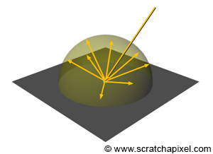

**Figure 3:** Diffuse surfaces reflect light equally in all directions contained within a hemisphere of directions oriented about the surface normal.

This is almost the complete formula to compute the color of a point on a diffuse surface, knowing the incident light energy, the surface normal, the light direction, and the surface albedo. We are only missing one term to complete the equation.

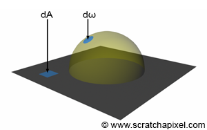
As mentioned in the first chapter, diffuse surfaces have a unique property in that they reflect light impinging on their surface equally in every direction above the point of incidence. Imagine a light beam striking the surface of an object at one point and light energy being redistributed over that point in a hemisphere of directions expanding from the point of incidence outward, as shown in Figure 3. From a practical perspective, this means that the energy of the light beam, which we know is attenuated by the cosine of the angle between the surface normal and the light direction, is redistributed across the surface of a hemisphere. We can look at this problem the other way around and say that if we were to collect all the energy distributed across the surface of this hemisphere, it should equal the incident light energy, minus, of course, the amount of light that was absorbed by the surface. There is as much light redistributed as light incident on the surface, minus the amount of light absorbed by the surface. Mathematically, collecting the light energy across the surface of the hemisphere can be written using an integral:

$$\text{Amount of Reflected Light(P)} = \color{green}{\int_\Omega} \color{red}{\rho_d \cdot \text{Light Energy} \cdot \cos\theta}\color{green}{\;d\omega}.$$

The integral symbol means that we are interested in summing up, in a way, all the light energy that is spread across the surface of the hemisphere (imagine that you are counting the number of photons distributed over the surface of that hemisphere). The concept of the hemisphere in this equation is represented by the term $\Omega$. Reading this equation, you could say, "collect (the $\int$ term) the light energy (aka the number of photons, for example) of an incident light beam reflected by the surface at $P$, over the hemisphere (defined here by the term $\Omega$) oriented about the surface normal $N$ at the point of incidence." We know that the energy reflected is itself equal to the albedo of the surface multiplied by the amount of incident light energy and the cosine of the angle between the surface normal and the light direction. So, if we put these two concepts together, we get the integral term on the left (the green part in the equation) and what we are trying to collect, which is the term in red on the right of the integral.

If you are not familiar with the concept of an integral, we advise you to read the lesson on The Mathematics of Shading.

**Figure 4:** A differential solid angle is to a sphere what a differential area is to a plane or an arbitrary surface.

We won't give much information about integrals in this lesson, nor explain what the term $d\omega$ means. However, you should know that collecting "some value" across the surface of some object (a half-sphere in this case) can be seen as just splitting the surface into small areas, measuring the quantity we are interested in over the surface of these small areas, and summing up the results. We do this because the quantity we want to measure might vary across the surface of the object. When an object is just a flat plane, for instance, the area of a patch on this plane can just be measured in terms of square meters, an inch, or whatever units you wish to use to measure lengths. We would call this a differential area. We already introduced this concept earlier in this chapter and mentioned that differential areas are generally denoted $dA$. However, when it comes to a sphere or a hemisphere, we don't use square meters but steradians instead. A steradian is the unit of solid angle, where a solid angle is a measure of a patch on a sphere expressed in terms of angle rather than length. The symbol used in CG for solid angle is most of the time $\omega$. The term $d\omega$ thus refers to the concept of a differential solid angle, or in more common terms, a very small patch on the sphere but expressed in terms of solid angle. The goal with the integral mentioned above is to measure some value (the value defined in red in our example) by splitting the surface of interest (a hemisphere in this case) into very small patches (the $d\omega$ over the surface of that hemisphere which, because they are patches on the surface of a half-sphere, are mathematically measured in terms of steradian), and summing up the value measured for each one of these small patches or differential solid angles.

Please refer to the lesson The Mathematics of Shading for more information on integrals and how they can be solved either analytically or using techniques such as Monte Carlo integration.

Now, hopefully, you will agree that the amount of light that is reflected by the surface can't be greater than the amount of light that is effectively reaching the surface minus the amount of light that is absorbed. Logical, right? In other terms, if we could measure the amount of energy reflected by the surface using the equation above, it should be lower than or equal to the amount of incident light energy:

$$ \text{Total Amount of Reflected Light(P)} = \color{green}{\int_\Omega} \color{red}{\rho_d \cdot L_i \cdot \cos\theta}\color{green}{\;d\omega} \le L_i . $$

Where $L_i$ here stands for the amount of incident light energy. Hopefully, for us, the result of the integral in this particular case can be computed analytically. To put it simply, we know what the result of this integral is. Again, refer to the lesson on The Mathematics of Shading to learn about how integrals can be solved. In this case, we can use the first fundamental theorem of calculus. The idea behind this theorem is that if you know the antiderivative $F$ of some function $f$, then it is possible to compute the result of the integral of $f$ over some closed intervals. This is often written as:

$$\int_a^b f(x)dx = F(b) - F(a).$$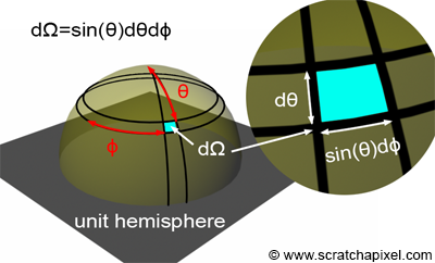

**Figure 5:** The differential solid angle can be defined in terms of the differential polar ($\theta$) and azimuthal ($\phi$) angles.

The problem with our integral is that it is expressed in terms of solid angle (the $d\omega$ term), which is not an easy unit to work with. To make things simpler, we can replace the term $d\omega$ with $\sin\theta d\theta d\phi$, where the angle $\theta$ (the Greek letter theta) is defined over the interval [0, $\pi/2$] and the angle $\phi$ (the Greek letter phi) is defined over the interval [0, $2\pi$]. This idea is illustrated in Figure 5. In other words, rather than using steradians, we now use radians or angles, which are easier to deal with. Though we now have to integrate over two quantities, $\theta$ and $\phi$, which means that we need two integrals instead of one:

Where does the use of $\sin(\theta)$ in the conversion from solid angles to using the angles $\theta$ and $\phi$ in spherical coordinates come from?

It comes from the need to account for the varying "width" of the area on the sphere's surface as $\theta$ changes. This is a fundamental concept in spherical geometry, especially when describing areas on a sphere using integral calculus.

Spherical coordinates ($\theta$ and $\phi$) represent points in three dimensions on the unit sphere (radius = 1). In this system:

$\theta$ (theta) is the polar angle, measured from the positive z-axis.
$\phi$ (phi) is the azimuthal angle, measured in the xy-plane from the positive x-axis.

When dealing with integrals over surfaces like spheres, we express areas in terms of solid angles. A solid angle $d\omega$ in spherical coordinates is related to the area on a unit sphere. When projecting a small area from the surface of a sphere (like a patch of area) onto the plane of $\theta$ and $\phi$, the actual area of that patch on the sphere is not just a simple rectangle due to the curvature of the sphere. As $\theta$ varies, especially away from the equator ($\theta = \frac{\pi}{2}$), the "width" of the bands of latitude decreases.

At the poles ($\theta = 0$ or $\theta = \pi$), the bands become point-like, having no width.
At the equator ($\theta = \frac{\pi}{2}$), the bands are at their maximum width.

The factor of $\sin(\theta)$ accounts for this change in width. It essentially scales the "horizontal" (or azimuthal) component of our spherical area element, which is proportional to $\sin(\theta)$.

The differential area element on a sphere (surface area) in spherical coordinates is given by $\sin(\theta) d\theta d\phi$. The integral for a function over the sphere would then be expressed as:

$$ \int \int f(\theta, \phi) \sin(\theta) \, d\theta \, d\phi $$

This integral sums up the function $f$ over the spherical surface, correctly accounting for the varying area size at different latitudes due to $\sin(\theta)$. The usage of $\sin(\theta)$ is essential for accurately reflecting the geometrical reality of spherical surfaces. It ensures that the area elements represented in the integrals correctly account for the sphere’s geometry, where areas near the poles are smaller compared to those near the equator. This geometric correction is crucial when converting the integral from one in terms of solid angles to one involving the more familiar angular measures, $\theta$ and $\phi$.

Mathematical proof that this double integral is equal to the area of a unity sphere:

Let's perform the integration. The integral to find the total surface area of the sphere is:

$$ A = \int_{0}^{2\pi} \int_{0}^{\pi} \sin(\theta) \, d\theta \, d\phi $$

Integrate over $\theta$:
$$ \int_{0}^{\pi} \sin(\theta) \, d\theta = -\cos(\theta) \bigg|_{0}^{\pi} = -\cos(\pi) + \cos(0) = 2 $$
Integrate over $\phi$:
$$ \int_{0}^{2\pi} d\phi = 2\pi $$

Combining these results:

$$ A = 2 \times 2\pi = 4\pi $$

This result, $4\pi$, is exactly the formula for the surface area of a unit sphere, confirming that the integral calculation using $\sin(\theta)$ in the area element correctly yields the total area.

$$ {\int_{\phi=0}^{2\pi}}{ \int_{\theta=0}^{\pi/2}} \rho_d \cdot L_i \cdot \cos\theta \cdot \sin\theta \; {d\phi} \; {d\theta} \le L_i. $$

What we integrate over in an integral are the quantities that, at the end of the equations, are preceded by the letter $d$. In this example, this would be $\phi$ and $\theta$. In other words, the constants $\rho_d$ and $L_i$ are not affected and can be taken out of the integrals:

$$ \rho_d \cdot L_i {\int_{\phi=0}^{2\pi}}{ \int_{\theta=0}^{\pi/2}} \cos\theta \cdot \sin\theta \; {d\phi} \; {d\theta} \le L_i. $$

Note also that we have the terms $L_i$ on both sides of the $\le$ sign. If we divide both sides of the inequality by $L_i$, we get:

$$ \rho_d \cdot \dfrac{L_i}{L_i} {\int_{\phi=0}^{2\pi}}{ \int_{\theta=0}^{\pi/2}} \cos\theta \cdot \sin\theta \; {d\phi} \; {d\theta} = \rho_d {\int_{\phi=0}^{2\pi}}{ \int_{\theta=0}^{\pi/2}} \cos\theta \cdot \sin\theta \; {d\phi} \; {d\theta} \le 1. $$

Also:

$$\int_a^b dx = b - a.$$

Thus:

$$\int_0^{2\pi} d\phi = 2\pi.$$

We can replace the first integral (the integral over $\phi$) by $2\pi$:

$$\rho_d \cdot 2 \pi {\int_{\theta=0}^{\pi/2}} \cos\theta \cdot \sin\theta \; {d\theta} \le 1.$$

We can finally use the first fundamental theorem of calculus to solve the last integral. The antiderivative of $\cos x \sin x$ is:

$$-\dfrac{1}{2}\cos^2(x).$$

Just in case you didn't understand how the antiderivative was determined, here are the steps. We will start from the antiderivative and demonstrate that its derivative is indeed $\cos(x) \sin(x)$:

Starting Expression:
- Consider the function $-\frac{1}{2} \cos^2(x)$.
Define the Inner Function:
- Define $u = \cos(x)$. This choice leads us to re-examine the expression: $-\frac{1}{2} u^2$.
Apply the Chain Rule:
- To differentiate $-\frac{1}{2} u^2$ with respect to $x$, we utilize the chain rule. The chain rule stipulates that to differentiate a composite function, you first differentiate the outer function treating the inner function as a constant, and then multiply by the derivative of the inner function with respect to $x$.
Chain Rule in Action:
- Differentiating $-\frac{1}{2} u^2$ with respect to $u$ yields $-u$.
- The derivative of $u = \cos(x)$ with respect to $x$, given $u = \cos(x)$, is $-\sin(x)$.
Combining the Results:
- The derivative thus becomes $-u \times (-\sin(x)) = \cos(x) \sin(x)$.
Final Step:
- By substituting back into the original expression and considering the steps, we find:
$$\frac{d}{dx}\left(-\frac{1}{2} \cos^2(x)\right) = \cos(x) \sin(x).$$
- This confirms that the derivative of $-\frac{1}{2} \cos^2(x)$ is indeed $\cos(x) \sin(x)$, verifying that $-\frac{1}{2} \cos^2(x)$ is the correct antiderivative.

Thus:

$$ \int_0^{\pi/2} \cos\theta \cdot \sin\theta \; {d\theta} = \left [ -\dfrac{1}{2}\cos^2(x) \right ]_0^{\pi/2} = -\dfrac{1}{2}\cos^2(\pi/2) + \dfrac{1}{2}\cos^2(0) = 0 + \dfrac{1}{2} = \dfrac{1}{2}. $$

Finally, we get the result:

$$\rho_d \cdot 2 \pi \cdot \dfrac{1}{2} = \rho_d \cdot \pi \le 1.$$

The term $\rho_d$, the surface albedo, can take any value in the range [0,1]. If we imagine that a surface has an albedo of, let's say, 0.5, then clearly the inequality above is not correct: $\frac{1}{2} \cdot \pi$ is not less than 1. So the equation we have above is not true for all possible values that the albedo can take on. The only solution for making this inequality work is to divide the albedo itself by $\pi$:

$$\dfrac{\rho_d}{\pi} \cdot \pi \le 1.$$

And this would work. So the amount of light reflected by a diffuse surface is in fact:

$$\text{Diffuse Surface Color} = \dfrac{\rho_d}{\pi} \cdot L_i \cdot \cos \theta.$$

Because if you integrate this equation over the hemisphere:

$$\text{Total Amount of Reflected Light(P)} = {\int_\Omega} {\dfrac{\rho_d}{\pi} \cdot L_i \cdot \cos\theta}{\;d\omega} \le L_i .$$

Then you indeed find out that with this equation, a diffuse surface cannot reflect more energy than it receives:

$${\rho_d}\le 1.$$

You can view the division of the albedo by $\pi$ as a method for normalizing the result of the integral.

Now that we know the equation, let's put this into practice. This time, we will need to add a light to the scene. For simplicity, we will start with a distant light and only one light. We will learn about what we should do when there is more than one light in the scene and about spherical lights in the next chapter. We will modify the source code of the ray tracer we developed in the previous lesson. First, each object in the scene now has an albedo parameter, which you can see as the color of the object:

class Object 
{ 
    Object(const Matrix44f &o2w, const Vec3f &c = 0.18) : objectToWorld(o2w), worldToObject(o2w.inverse()), albedo(c) 
    ... 
    Vec3f albedo; 
    ... 
};

Why is the default color 0.18? The reason we set the albedo default value to 0.18 is that objects from the real world reflect, on average, around 18% of the light they receive. This is an average value. In other words, if you look at how much light different fruits, asphalt, snow, tree leaves, grass, etc., reflect and take the average of all these values, you end up with a value close to 18%. More information on this topic can be found in the lesson A Creative Dive into BRDF, Linearity, and Exposure.

When a ray hits an object from the scene, we will first compute the surface normal at the intersection point. We then compute the pixel color associated with the camera ray using the equation we provided above:

Vec3f castRay( 
    const Vec3f &orig, const Vec3f &dir, 
    const std::vector<std::unique_ptr<Object>> &objects, 
    const std::unique_ptr<DistantLight> &light, 
    the Options &options) 
{ 
    Vec3f hitColor = options.backgroundColor; 
    float tnear = kInfinity; 
    Vec2f uv; 
    uint32_t index = 0; 
    Object *hitObject = nullptr; 
    if (trace(orig, dir, objects, tnear, index, uv, &hitObject)) { 
        Vec3f hitPoint = orig + dir * tnear; 
        Vec3f hitNormal; 
        Vec2f hitTexCoordinates; 
        hitObject->getSurfaceProperties(hitPoint, dir, index, uv, hitNormal, hitTexCoordinates); 
        Vec3f L = -light->dir; 
        // compute the color of a diffuse surface illuminated
        // by a single distant light source.
        hitColor = hitObject->albedo / M_PI * light->intensity * light->color * std::max(0.f, hitNormal.dotProduct(L)); 
    } 
 
    return hitColor; 
}

This is just a straightforward application of the equation. The albedo is divided by $\pi$, which ensures that the surface doesn't reflect more light than it receives. Then the result is multiplied by the light intensity, which is further multiplied by the light color (this gives the total amount of light energy incident at the intersection point), attenuated by the cosine of the angle between the surface normal at the intersection point and the light direction.

Note that if the light and the surface normal are on the same side of the plane perpendicular to the surface normal, then the result of the dot product between the surface normal and the light direction is positive. However, if the light is "behind" the surface, the result of the dot product is negative. Of course, if the light is technically behind the surface, it shouldn't illuminate the surface anymore, but more importantly, we don't want to introduce negative values in the computation of the surface color. Thus, we clamp the result of the dot product using the C++ std::max() function (line 20).

Here are some results:

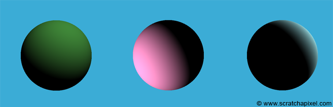
Congratulations! You now know about two shading techniques. You know about the facing ratio and simulating the appearance of the perfect diffuse surface. In the next chapter, we will learn about handling more than one light source as well as using spherical lights. We will also learn about adding shadows to the image.