Introduction to Shading

Spherical Light

Reading time: 11 mins.

As mentioned in the previous chapter, this is merely a high-level introduction to light and shadows. Readers interested in studying this topic further are invited to read the lessons A Creative Dive into BRDF, Linearity, and Exposure and Introduction to Lighting. While these lessons are also part of the beginner section, they delve deeper into the topic of light implementation. You can then continue with the lessons from the advanced section.

Structure of this Chapter

In this chapter, we will learn how to simulate spherical (or point) lights and how to cast shadows with spherical lights.

Spherical Lights

We have already introduced the concept of directional light sources, which can be used to simulate distant light sources such as the sun. Directional sources are light sources that are so far away from the scene that the light rays they emit can be considered parallel to each other. In other words, a distant light source emits rays in a single direction.

**Figure 1:** Compute the light direction for point light sources.

Spherical light sources are different. They are not distant like directional light sources but local. A spherical light can be represented as a single point of light in 3D space from which light is emitted radially from the point of emission. For this reason, they are also frequently called point light sources. Point light sources can be used to simulate things such as the flame of a candle or a light bulb. Although, as mentioned in the chapter on directional light sources, spherical or point light sources are also considered light sources with no size. In other words, we model them as an ideal point in space from which light is emitted radially, but such an object does not exist in nature. The flame of a candle or a light bulb may well emit light radially, though they have a size. This is not a problem right now, but keep in mind that so far, our lights are considered to be infinitesimally small in size. Such light sources are often referred to as delta lights, as explained in the introductory chapter on lights. When spherical lights emit light equally in all directions, we say they are isotropic.

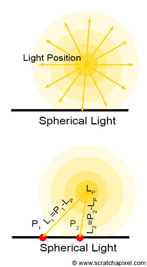
How do we simulate point light sources? First, we need to consider the way light is emitted: radially. From a coding perspective, this can be simulated by simply tracing a line from the point that is being shaded ($P$) to the spherical light position. This line will indicate the direction of the light ray emitted by the point light source towards $P$, as shown in Figure 1.

From a coding perspective, all we need to do to define a point light source is to add a member variable to the Light base class to keep track of its position in space. We will assume that the point light source is created at the origin of the world coordinate system. To modify its position in 3D space, we will use the light-to-world transformation matrix (as we did to modify the directional light source's direction):

class PointLight : public Light 
{ 
public: 
    Vec3f pos;  // Position of the light in world space
    PointLight(const Matrix44f &l2w, const Vec3f &c = 1, const float &i = 1) : Light(l2w, c, i) 
    { l2w.multVecMatrix(Vec3f(0), pos); } 
};

Since the light direction depends on the position of $P$ and the position of the light source in 3D space, we will add a getDirection() function to the Light base class. This function will take the point $P$ as an argument and return a normalized light direction. For directional light sources, this direction is constant. For spherical light sources, it must be computed explicitly:

class PointLight : public Light 
{ 
public: 
    Vec3f pos; // Position of the light
    PointLight(const Matrix44f &l2w, the Vec3f &c = 1, the float &i = 1) : Light(l2w, c, i) 
    { l2w.multVecMatrix(Vec3f(0), pos); } 
    // P: is the shaded point
    Vec3f getDirection(const Vec3f &P) const { return (pos - P).normalize(); } 
};

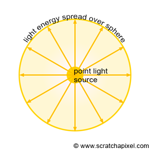
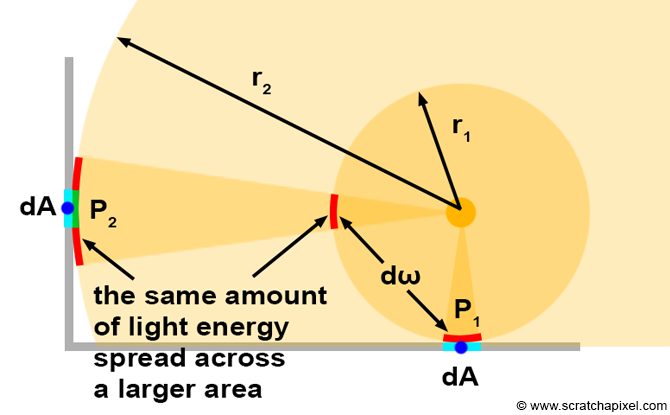
**Figure 2:** Light energy emitted from a point light source is distributed across the surface of a sphere of radius $r$. This is, of course, an infinity of such spheres centered around the point light position.

Spherical light sources differ from directional light sources in one more aspect. Let's consider point light sources first. As mentioned earlier in this chapter, spherical light sources emit light from a single point in space. The light energy emitted from that point is distributed across the surface of a sphere, as shown in Figure 2. Without delving into the details (which would involve a more thorough understanding of radiometry), let's simply state for now that the entire light energy or power of the point light source is redistributed over that sphere. As with diffuse surfaces, the amount of light arriving on a small differential area $dA$ is somewhat proportional to the amount of light contained within a small patch of the sphere with radius $r_1$, roughly equal in area to $dA$, as shown in the illustration below. However, as you can see in the same illustration, as the sphere expands, the area of the differential solid angle $d\omega$ that matched the area of the differential area $dA$ also increases. In other words, the energy that was concentrated over $d\omega$ is now spread across a much larger area. Consequently, $P_2$ receives less light than $P_1$, or to put it differently, $P_2$ will appear darker than $P_1$ (the amount of light $P_2$ receives is proportional to the green solid angle over the red solid angle).

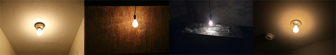
This effect can easily be observed with any real point light source, such as a light bulb. Objects that are closer to the source are brighter. The contribution of the light seems to decrease as the distance from the light source to the objects increases. The question now is to determine what governs this falloff.

The amount of light energy arriving at a point in the scene from a point light source depends on the area of the "sphere," which itself depends on the sphere's radius. Note that this sphere doesn't actually exist; we use this image merely to help you visualize the process. When we speak of a sphere, what we actually mean is a sort of virtual sphere centered around the point of light source origin, with a radius equal to the distance from the point of the light source to $P$, a point in the scene that we wish to shade. What we are trying to determine is how much light arrives at $P$ from that point of light source. As suggested, the contribution of the point light source depends on the area of the sphere of radius $r$:

$$A = 4\pi r^2.$$

The intensity of the light arriving at $P$ is inversely proportional to the sphere's area. In other words:

$$L_i = \dfrac{\text{light intensity * light color}}{4 \pi r^2}.$$

For a more formal explanation, please refer to the lesson on radiometry.

Where $r$ is equal to the distance between the light position and $P$. This falloff is known in CG as the square falloff. Note that when the radius of the sphere doubles (if the distance between the point light source and $P$ doubles), the area of the sphere is multiplied by 4, and thus the light contribution is four times smaller. More generally, this kind of light attenuation follows what we call the inverse-square law. The profile of this falloff can be seen in the following figure.

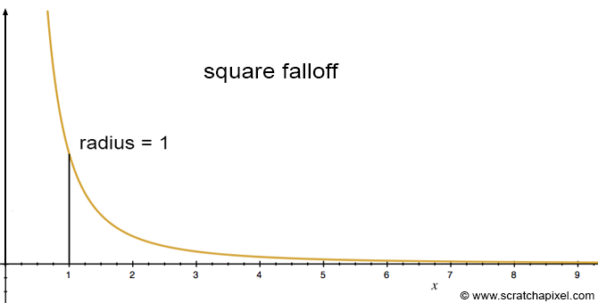
As you can observe from this graph, the contribution of a point light source decreases very rapidly with distance.

To implement this square falloff, we will make a small modification to the getDirection method, which we will rename getDirectionAndIntensity. As you may have guessed, this is also where we will compute the light intensity for a given $P$. We do so because we already compute in the method the vector connecting the light to $P$ to compute the light direction. We can use the square of this vector's length to attenuate the light intensity according to the inverse square law (line 13):

class PointLight : public Light 
{ 
    Vec3f pos; // Position of the light
public: 
    PointLight(const Matrix44f &l2w, const Vec3f &c = 1, const float &i = 1) : Light(l2w, c, i) 
    { l2w.multVecMatrix(Vec3f(0),

 pos); } 
    // P: is the shaded point
    void getDirectionAndIntensity(const Vec3f &P, Vec3f &lightDir, Vec3f &lightIntensity) const 
    { 
        lightDir = pos - P;  // Compute light direction 
        float r2 = lightDir.norm(); 
        lightDir.normalize(); 
        lightIntensity = intensity * color / (4 * M_PI * r2); 
    } 
};

Spherical Lights & Shadows

Computing shadows with spherical lights is quite straightforward. We can use similar techniques as those used for distant light sources. We simply need to compute the light direction and trace a ray in the opposite direction. Computing the light direction is straightforward: we trace a line from the light source to $P$, the shaded point. By normalizing the resulting vector, we obtain the light direction:

class PointLight : public Light 
{ 
    Vec3f pos; 
public: 
    PointLight(const Matrix44f &l2w, const Vec3f &c = 1, const float &i = 1) : Light(l2w, c, i) 
    { l2w.multVecMatrix(Vec3f(0), pos); } 
    // P: is the shaded point
    void getDirectionAndIntensity(const Vec3f &P, Vec3f &lightDir, Vec3f &lightIntensity) const 
    { 
        lightDir = pos - P; 
        float r2 = lightDir.norm(); 
        lightDir.normalize(); 
        lightIntensity = intensity * color / (4 * M_PI * r2); 
    } 
};

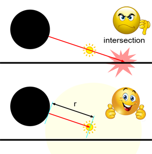
**Figure 3:** Any intersection whose distance is greater than the distance between $P$ and the light can be ignored.

However, there is a caveat. Directional lights, by definition, are extremely far away—considered to be at infinity. This is not the case with spherical lights. If we trace a shadow ray in the direction of the light, this ray could very well overshoot the point light source and intersect an object further away than the source. This would incorrectly suggest that the point is in shadow when, in fact, $P$ and the light are visible to each other (as shown in Figure 3). The solution to this problem is to set the ray's maximum length, or $tNear$, to the distance between $P$ and the light position (the distance we denoted $r$). That way, the trace() function will never accept an intersection whose distance is greater than $r$. In other words, if an intersection is found but the intersection distance is further away than the distance between $P$ and the light, then it will be ignored. Since we already computed the square of that distance in the getDirectionAndIntensity() function, we will just add a variable to the method that will be set to the distance between $P$ and the light:

class PointLight : public Light 
{ 
    Vec3f pos; 
public: 
    PointLight(const Matrix44f &l2w, const Vec3f &c = 1, const float &i = 1) : Light(l2w, c, i) 
    { l2w.multVecMatrix(Vec3f(0), pos); } 
    // P: is the shaded point
    void getShadingInfo(const Vec3f &P, Vec3f &lightDir, Vec3f &lightIntensity, float &dist) const 
    { 
        lightDir = pos - P; 
        // Compute the square distance
        float r2 = lightDir.norm(); 
        dist = sqrtf(r2); 
        // Normalize the incident light ray direction
        lightDir.x /= dist, lightDir.y /= dist, lightDir.z /= dist; 
        // Apply square falloff
        lightIntensity = intensity * color / (4 * M_PI * r2); 
    } 
};

Then we will set the shadow ray $tNear$ variable to the result of dist. This can be done directly if we pass the isectShad.tNear variable directly to the getShadingInfo() method of the light (we can change the method's name in the process to make it more generic).

IsectInfo isectShad; 
light->getShadingInfo(hitPoint, lightDir, lightIntensity, isectShad.tNear); 
bool vis = !trace(hitPoint + hitNormal * options.bias, -lightDir, objects, isectShad, kShadowRay);

What's Next?

We can now simulate diffuse surfaces and the effects of directional and point light sources. However, so far, we have only rendered scenes containing one light source. How we can extend the technique to multiple light sources will be the topic of the next chapter.