Mathematics of Computing the 2D Coordinates of a 3D Point
Reading time: 39 mins.Finding the 2D Pixel Coordinates of a 3D Point: Explained from Beginning to End
When a point or vertex is defined in a scene and is visible to the camera, it appears in the image as a dot—or more precisely, as a pixel if the image is digital. We've already discussed the perspective projection process, which is used to convert the position of a point in 3D space to a position on the image surface. However, this position is not yet expressed in terms of pixel coordinates. How then do we determine the final 2D pixel coordinates of the projected point in the image? In this chapter, we will review the process of converting points from their original world position to their final raster position (their position in the image in terms of pixel coordinates).
The technique we will describe in this lesson is specific to the rasterization algorithm, the rendering technique used by GPUs to produce images of 3D scenes. If you want to learn how it is done in ray-tracing, check out the lesson Ray-Tracing: Generating Camera Rays.
World Coordinate System and World Space
When a point is first defined in a scene, its coordinates are specified in world space: the coordinates of this point are described with respect to a global or world Cartesian coordinate system. This system has an origin, known as the world origin, and the coordinates of any point defined in this space are described in relation to this origin—the point whose coordinates are [0,0,0]. Points are expressed in world space (Figure 1).
4x4 Matrix Visualized as a Cartesian Coordinate System
Objects in 3D can be transformed using three operators: translation, rotation, and scale. If you recall our discussions from the lesson dedicated to Geometry, you'll remember that linear transformations — any combination of these three operators — can be represented by a 4x4 matrix. If you are unsure why and how this works, consider revisiting the lesson on Geometry, particularly the chapters: How Does Matrix Work Part 1 and Part 2. In these matrices, the first three coefficients along the diagonal encode the scale (coefficients c00, c11, and c22), the first three values of the last row encode the translation (coefficients c30, c31, and c32 — assuming the row-major order convention), and the 3x3 upper-left inner matrix encodes the rotation (the coefficients colored in red, green, and blue).
$$ \begin{bmatrix} \color{red}{c_{00}}& \color{red}{c_{01}}&\color{red}{c_{02}}&\color{black}{c_{03}}\\ \color{green}{c_{10}}& \color{green}{c_{11}}&\color{green}{c_{12}}&\color{black}{c_{13}}\\ \color{blue}{c_{20}}& \color{blue}{c_{21}}&\color{blue}{c_{22}}&\color{black}{c_{23}}\\ \color{purple}{c_{30}}& \color{purple}{c_{31}}&\color{purple}{c_{32}}&\color{black}{c_{33}}\\ \end{bmatrix} \begin{array}{l} \rightarrow \quad \color{red} {x-axis}\\ \rightarrow \quad \color{green} {y-axis}\\ \rightarrow \quad \color{blue} {z-axis}\\ \rightarrow \quad \color{purple} {translation}\\ \end{array} $$When examining the coefficients of a matrix, it can be challenging to discern precisely what the scaling or rotation values are because rotation and scale are combined within the first three coefficients along the diagonal of the matrix. For now, let's focus solely on rotation and translation.
As depicted, we have nine coefficients representing a rotation. But how can we interpret what these nine coefficients actually represent? Until now, our discussion has revolved around matrices, but let's now shift our focus to coordinate systems. We will connect the two concepts — matrices and coordinate systems — to enhance understanding.
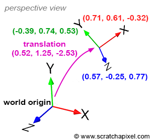
The only Cartesian coordinate system we have discussed so far is the world coordinate system. This system is a convention used to define the coordinates [0,0,0] in our 3D virtual space along with three unit axes that are orthogonal to each other, as shown in Figure 1. It acts as the prime meridian of a 3D scene — any other point or arbitrary coordinate system in the scene is defined with respect to the world coordinate system. Once this system is established, we can create other Cartesian coordinate systems. Like points, these systems are characterized by a position in space (a translation value) and three unit axes or vectors that are orthogonal to each other, which are the defining features of Cartesian coordinate systems. Both the position and the values of these three unit vectors are defined with respect to the world coordinate system, as depicted in Figure 1.
In Figure 1, the purple coordinates denote the position, while the coordinates of the x, y, and z axes are in red, green, and blue respectively. These colors represent the axes of an arbitrary coordinate system, all defined in relation to the world coordinate system. Importantly, the axes that make up this arbitrary coordinate system are unit vectors.
The upper-left 3x3 portion of our 4x4 matrix contains the coordinates of our arbitrary coordinate system's axes. Since we have three axes, each with three coordinates, this results in nine coefficients. If the 4x4 matrix stores its coefficients using the row-major order convention (as is the case with Scratchapixel), then:
-
The first three coefficients of the matrix's first row (c00, c01, c02) correspond to the coordinates of the x-axis.
-
The first three coefficients of the matrix's second row (c10, c11, c12) correspond to the coordinates of the y-axis.
-
The first three coefficients of the matrix's third row (c20, c21, c22) correspond to the coordinates of the z-axis.
-
The first three coefficients of the matrix's fourth row (c30, c31, c32) correspond to the translation values of the coordinate system's position.
Consider this example of a transformation matrix for the coordinate system shown in Figure 1:
$$ \begin{bmatrix} \color{red}{+0.718762}&\color{red}{+0.615033}&\color{red}{-0.324214}&0\\ \color{green}{-0.393732}&\color{green}{+0.744416}&\color{green}{+0.539277}&0\\ \color{blue}{+0.573024}&\color{blue}{-0.259959}&\color{blue}{+0.777216}&0\\ \color{purple}{+0.526967}&\color{purple}{+1.254234}&\color{purple}{-2.532150}&1\\ \end{bmatrix} \begin{array}{l} \rightarrow \quad \color{red} {x-axis}\\ \rightarrow \quad \color{green} {y-axis}\\ \rightarrow \quad \color{blue} {z-axis}\\ \rightarrow \quad \color{purple} {translation}\\ \end{array} $$In conclusion, a 4x4 matrix represents a coordinate system, and reciprocally, a 4x4 matrix can represent any Cartesian coordinate system. It's essential to always perceive a 4x4 matrix as a coordinate system, and vice versa. We often refer to this as a "local" coordinate system in relation to the "global" coordinate system, which in our discussions, is the world coordinate system.
Local vs. Global Coordinate System

Having established how a 4x4 matrix can be interpreted and introduced the concept of a local coordinate system, let's delve into what local coordinate systems are used for. By default, the coordinates of a 3D point are defined with respect to the world coordinate system. The world coordinate system is just one among an infinite number of possible coordinate systems. However, we need a standard system to measure everything against by default, hence the creation of the "world coordinate system" (it is a convention, like the Greenwich Meridian, where longitude is defined to be 0). Having one reference point is useful but not always the best way to track positions in space. For instance, if you are looking for a house on a street, knowing the house's longitude and latitude coordinates would allow you to find it using GPS. However, if you are already on that street, finding the house using its street number is simpler and quicker than using GPS. A house number is a coordinate defined with respect to a reference point—the first house on the street. In this context, the street numbers function as a local coordinate system, while the longitude/latitude coordinate system acts as a global coordinate system. Although street numbers can be defined with respect to the global coordinate system, they are primarily represented with their coordinates relative to a local reference: the first house on the street. Local coordinate systems are particularly useful for finding things when you are within the frame of reference in which these things are defined (e.g., when you are on the street itself). It's also important to note that the local coordinate system can be described with respect to the global coordinate system (for instance, we can determine its origin in terms of latitude/longitude coordinates).
This principle applies similarly in computer graphics (CG). It's always possible to determine the location of things relative to the world coordinate system, but to simplify calculations, it is often convenient to define things relative to a local coordinate system (we will illustrate this with an example further down). This is the primary purpose of "local" coordinate systems.
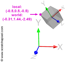
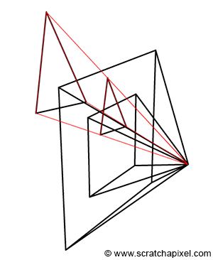
When you move a 3D object in a scene, such as a cube (although this applies regardless of the object's shape or complexity), the transformations applied to that object (translation, scale, and rotation) can be represented by what we call a 4x4 transformation matrix. This matrix is essentially a 4x4 matrix, but since it's used to change the position, scale, and rotation of that object in space, we refer to it as a transformation matrix. This 4x4 transformation matrix can be regarded as the object's local frame of reference or local coordinate system. In essence, you don't transform the object itself; instead, you transform the local coordinate system of that object. Since the vertices making up the object are defined with respect to that local coordinate system, moving the coordinate system consequently moves the object's vertices along with it (as shown in Figure 3). It's crucial to understand that we don't explicitly transform the coordinate system; rather, we translate, scale, and rotate the object. A 4x4 matrix represents these transformations, and this matrix can be visualized as a coordinate system.
Transforming Points from One Coordinate System to Another
The coordinates of a house, whether expressed as its address or its longitude/latitude, will differ, although it is the same physical location. These differences arise because the coordinates relate to the frame of reference within which the house’s location is defined. Consider the highlighted vertex in Figure 3. In the local coordinate system, this vertex's coordinates are \([-0.5, 0.5, -0.5]\). However, in "world space" (when coordinates are defined with respect to the world coordinate system), the coordinates become \([-0.31, 1.44, -2.49]\). Different coordinates, same point.
As suggested earlier, it is often more convenient to operate on points when they are defined with respect to a local coordinate system rather than the world coordinate system. For example, with the cube in Figure 3, representing the corners in local space is simpler than representing them in world space. But how do we convert a point or vertex from one coordinate system to another? This transformation is a common process in computer graphics (CG) and is straightforward. Suppose we know the 4x4 matrix \(M\) that transforms a coordinate system \(A\) into a coordinate system \(B\). In that case, if we transform a point whose coordinates are initially defined with respect to \(B\) using the inverse of \(M\) (the reason for using the inverse of \(M\) rather than \(M\) itself will be explained next), we obtain the coordinates of the point \(P\) with respect to \(A\).
Let's explore an example using Figure 3. The matrix \(M\) that transforms the local coordinate system to which the cube is attached is:
$$ \begin{bmatrix} \color{red}{+0.718762}&\color{red}{+0.615033}&\color{red}{-0.324214}&0\\ \color{green}{-0.393732}&\color{green}{+0.744416}&\color{green}{+0.539277}&0\\ \color{blue}{+0.573024}&\color{blue}{-0.259959}&\color{blue}{+0.777216}&0\\ \color{purple}{+0.526967}&\color{purple}{+1.254234}&\color{purple}{-2.532150}&1\\ \end{bmatrix} $$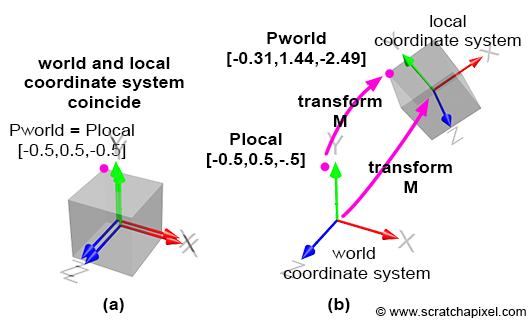
By default, the local coordinate system coincides with the world coordinate system; the cube vertices are defined with respect to this local coordinate system. This is illustrated in Figure 4a. Then, we apply the matrix \( M \) to the local coordinate system, which changes its position, scale, and rotation, depending on the matrix values. This is illustrated in Figure 4b. Before we apply the transformation, the coordinates of the highlighted vertex in Figures 3 and 4 (the purple dot) are the same in both coordinate systems, since the frames of reference coincide. However, after the transformation, the world and local coordinates of the points differ, as shown in Figures 4a and 4b. To calculate the world coordinates of that vertex, we need to multiply the point's original coordinates by the local-to-world matrix; we call it local-to-world because it defines the coordinate system with respect to the world coordinate system. This process is logical: if you transform the local coordinate system and want the cube to move with this coordinate system, you apply the same transformation that was applied to the local coordinate system to the cube vertices. To do this, multiply the cube's vertices by the local-to-world matrix (denoted \( M \) here for simplicity):
$$P_{world} = P_{local} \times M$$To convert from world coordinates back to local coordinates, transform the world coordinates using the inverse of \( M \):
$$P_{local} = P_{world} \times M^{-1}$$In mathematical notation, this is expressed as:
$$ \begin{array}{l} P_{world} = P_{local} \times M_{local-to-world}\\ P_{local} = P_{world} \times M_{world-to-local} \end{array} $$Let's verify this. The coordinates of the highlighted vertex in local space are \([-0.5, 0.5, 0.5]\) and in world space: \([-0.31, 1.44, -2.49]\). We also know the matrix \( M \) (local-to-world). If we apply this matrix to the point's local coordinates, we should obtain the point's world coordinates:
$$ \begin{array}{l} P_{world} = P_{local} \times M\\ P_{world}.x = P_{local}.x \times M_{00} + P_{local}.y \times M_{10} + P_{local}.z \times M_{20} + M_{30}\\ P_{world}.y = P_{local}.x \times M_{01} + P_{local}.y \times M_{11} + P_{local}.z \times M_{21} + M_{31}\\ P_{world}.z = P_{local}.x \times M_{02} + P_{local}.y \times M_{12} + P_{local}.z \times M_{22} + M_{32}\\ \end{array} $$Implement and check the results using the code from the Geometry lesson:
Matrix44f m(0.718762, 0.615033, -0.324214, 0, -0.393732, 0.744416, 0.539277, 0, 0.573024, -0.259959, 0.777216, 0, 0.526967, 1.254234, -2.53215, 1);
Vec3f Plocal(-0.5, 0.5, -0.5), Pworld;
m.multVecMatrix(Plocal, Pworld);
std::cerr << Pworld << std::endl;
The output is: (-0.315792, 1.4489, -2.48901).
Now, transform the world coordinates of this point back into local coordinates. Our implementation of the Matrix class includes a method to invert the current matrix. Use it to compute the world-to-local transformation matrix and then apply this matrix to the point's world coordinates:
Matrix44f m(0.718762, 0.615033, -0.324214, 0, -0.393732, 0.744416, 0.539277, 0, 0.573024, -0.259959, 0.777216, 0, 0.526967, 1.254234, -2.53215, 1);
m.invert();
Vec3f Pworld(-0.315792, 1.4489, -2.48901), Plocal;
m.multVecMatrix(Pworld, Plocal);
std::cerr << Plocal << std::endl;
The output is: (-0.500004, 0.499998, -0.499997).
The coordinates are not precisely \([-0.5, 0.5, -0.5]\) due to some floating point precision issues and because we've truncated the input point's world coordinates, but rounding to one decimal place, we get \([-0.5, 0.5, -0.5]\), which is the correct result.
At this point in the chapter, you should understand the difference between the world/global and local coordinate systems and how to transform points or vectors from one system to the other (and vice versa).
Camera Coordinate System and Camera Space

A camera in CG (computer graphics) and the natural world functions similarly to any 3D object. When taking a photograph, you must move and rotate the camera to adjust the viewpoint. Essentially, when you transform a camera (by translating and rotating it—note that scaling a camera doesn't make much sense), you are transforming a local coordinate system, which implicitly represents the transformations applied to that camera. In CG, this spatial reference system is referred to as the camera coordinate system (sometimes called the eye coordinate system in other sources). The significance of this coordinate system will be explained shortly.
A camera is fundamentally a coordinate system. Therefore, the technique we described earlier for transforming points from one coordinate system to another can also be applied here to transform points from the world coordinate system to the camera coordinate system (and vice versa). We say that we transform points from world space to camera space (or from camera space to world space if we apply the transformation the other way around).
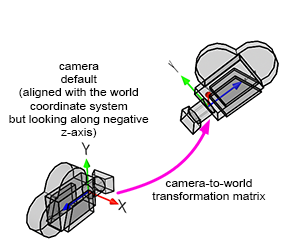
However, cameras are always aligned along the world coordinate system's negative z-axis. In Figure 5, you can observe that the camera's z-axis points in the opposite direction to the world coordinate system's z-axis (when the x-axis points to the right and the z-axis extends inward into the screen rather than outward).
Cameras are oriented along the world coordinate system's negative z-axis so that when a point is converted from world space to camera space (and later from camera space to screen space), if the point is to the left of the world coordinate system's y-axis, it will also map to the left of the camera coordinate system's y-axis. We need the x-axis of the camera coordinate system to point to the right when the world coordinate system x-axis also points to the right; the only way to achieve this configuration is by having the camera face down the negative z-axis.
Due to this orientation, the sign of the z-coordinate of points is inverted when transitioning from one system to the other. This is an important consideration when studying the perspective projection matrix.
To summarize: if we want to convert the coordinates of a point in 3D from world space (which is the space in which points are defined in a 3D scene) to the space of a local coordinate system, we need to multiply the point's world coordinates by the inverse of the local-to-world matrix.
The Importance of Converting Points to Camera Space
This section involves a lot of reading, but for a good reason. We will now demonstrate that to "project" a point onto the canvas (the 2D surface on which we will draw an image of the 3D scene), it is essential to convert or transform points from the world to camera space. Here's why.
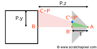
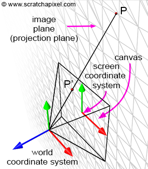
Let's revisit our goal: we aim to compute P', the coordinates of a point P from the 3D scene, on the surface of a canvas. This surface, where the image of the scene will be drawn, is also referred to as the projection plane, or in computer graphics, the image plane. If you trace a line from P to the eye (the origin of the camera coordinate system), P' is where this line intersects the canvas (as shown in Figure 7). When the coordinates of point P are defined with respect to the camera coordinate system, computing the position of P' becomes straightforward. If you observe Figure 7, which displays a side view of our setup, you'll notice we can draw two triangles \(\triangle ABC\) and \(\triangle AB'C'\), where:
-
A represents the eye.
-
B is the distance from the eye to point P along the camera coordinate system's z-axis.
-
C is the distance from the eye to P along the camera coordinate system's y-axis.
-
B' is the distance from the eye to the canvas (we will assume this distance is 1 to simplify our calculations).
-
C' is the distance from the eye to P' along the camera coordinate system's y-axis.
The triangles \(\triangle ABC\) and \(\triangle AB'C'\) are said to be similar (similar triangles have the same shape but different sizes). Similar triangles share a crucial property: the ratio between their corresponding sides is the same. Specifically:
$${ BC \over AB } = { B'C' \over AB' }.$$Given that the canvas is 1 unit away from the origin, we can set AB' equal to 1. We also know the positions of B and C, which are the z- (depth) and y-coordinate (height) of point P (assuming P's coordinates are defined in the camera coordinate system). Substituting these values into the equation gives us:
$${ P.y \over P.z } = { P'.y \over 1 }.$$Where y' is the y-coordinate of P'. Therefore:
$$P'.y = { P.y \over P.z }.$$This equation represents one of the simplest and most fundamental relationships in computer graphics, known as the z or perspective divide. The same principle applies to the x-coordinate. The projected point's x-coordinate (x') is calculated as the x-coordinate of the corner divided by its z-coordinate:
$$P'.x = { P.x \over P.z }.$$We've discussed this method in previous lessons, but it's important to demonstrate here that to compute P' using these equations, the coordinates of P must be defined with respect to the camera coordinate system. However, points from the 3D scene are initially defined with respect to the world coordinate system. Therefore, the first and essential operation we need to apply to points before projecting them onto the canvas is to convert them from world space to camera space.
How do we accomplish this? Suppose we know the camera-to-world matrix (similar to the local-to-camera matrix we studied previously). In that case, we can transform any point (whose coordinates are defined in world space) to camera space by multiplying this point by the inverse of the camera-to-world matrix (the world-to-camera matrix):
$$P_{camera} = P_{world} \times M_{world-to-camera}.$$With the point now in camera space, we can "project" it onto the canvas using the previously presented equations:
$$ \begin{array}{l} P'.x = \dfrac{P_{camera}.x}{P_{camera}.z}\\ P'.y = \dfrac{P_{camera}.y}{P_{camera}.z} \end{array} $$Remember, cameras typically align along the world coordinate system's negative z-axis. Readers in the past have been confused about this part of the lesson because the way it was written suggested that to orient the camera along the negative z-axis, we used a transformation matrix that would flip the camera's z-axis in addition to the camera-to-world matrix. Although this would technically be a valid approach, this is not how it's typically done. We do not explicitly flip the camera's z-axis. This can be observed if you examine what happens with the matrix of a camera in 3D software such as Maya. When you create a camera, it is by default oriented along the negative z-axis. However, if you query the camera's matrix, you will see that you get the identity matrix. What most (if not all) 3D software does is assume that matrices applied to cameras are just standard matrices for a right-hand coordinate system (for software like Maya, at least, and for our code, since we follow the same convention). The matrices used are the same type used to transform objects. There's nothing special or unusual about them. They are literally the same.
Let's consider an example. Imagine you have a point whose coordinates are (0,0,-10). Now imagine we moved the default camera (with no rotation) to position (1,0,2). If you apply this camera matrix (1 0 0 0 0 1 0 0 0 0 1 0 0 0 2 1) to our point, the new position with respect to the camera will be (1,0,-12). As you can see, the point's z-coordinate is negative. When we apply the z-divide to that point, the projected x-coordinate \(P'.x\) will be \(\frac{1}{-12}\). Its position along the x-axis will be negative, indicating that the point, previously to the right of the frame's vertical middle, is now to the left. The projected point's coordinates are mirrored.
The perspective divide operation works the same regardless of whether the point in camera space is "in front" of the camera or "behind" it (regardless of the convention you are using for the camera's default orientation). But of course, in practice, we discard points that are behind the camera. However, since we want our camera to look along the negative z-axis by default, and we want a point with a positive x-coordinate to be projected to the right of the vertical line passing through the center of the image, we need to invert the sign of the point's z-coordinate. When we do so, the position of the projected point with respect to the vertical and horizontal lines (considering points with positive or negative y-coordinates) passing through the center of the image is preserved.
$$ \begin{array}{l} P'.x = \dfrac{P_{camera}.x}{-P_{camera}.z}\\ P'.y = \dfrac{P_{camera}.y}{-P_{camera}.z} \end{array} $$As you can see, we don't explicitly use a matrix to flip the z-coordinate. We simply invert the point's z-coordinate at the time of the perspective divide. The thing that may confuse users is that in 3D software, the camera is oriented along the negative z-axis. It's drawn that way. You might think that they have created a camera geometry oriented along the positive axis and they use a matrix to flip the camera's orientation along the z-axis (or even worse, apply a 180-degree rotation along the y-axis). Don't be fooled by what you see in the viewport. The camera is just drawn that way in the viewport to make it clear to the user that this is how the image will be generated. But there's no matrix applied to it to orient it that way. It's simply "drawn" that way. And the illusion works (the image is properly created when you look through the camera view), because the z-inversion is applied to the z-coordinate during the perspective divide.
To summarize: points in a scene are defined in the world coordinate space. To project them onto the surface of the canvas, however, we first need to convert the 3D point coordinates from world space to camera space (no flip applied here to the z-coordinate as explained above). This conversion is accomplished by multiplying the point's world coordinates by the inverse of the camera-to-world matrix. Here is the code for performing this conversion:
Matrix44f cameraToWorld(0.718762, 0.615033, -0.324214, 0, -0.393732, 0.744416, 0.539277, 0, 0.573024, -0.259959, 0.777216, 0, 0.526967, 1.254234, -2.53215, 1);
Matrix44f worldToCamera = cameraToWorld.inverse();
Vec3f Pworld(-0.315792, 1.4489, -2.48901), Pcamera;
worldToCamera.multVecMatrix(Pworld, Pcamera);
std::cerr << Pcamera << std::endl;
With the point now in camera space, we can accurately compute its 2D coordinates on the canvas using the perspective projection equations, specifically by dividing the point's coordinates by the inverse of the point's z-coordinate.
A small note regarding GPUs, just in case you wonder if we are applying this process just for the sake of this lesson or if this is indeed what happens when you play your favorite video games. It turns out that this is exactly how GPUs render your games. We need to pass what we call the world-to-camera matrix and another type of matrix called the perspective matrix to the vertex shader. Now, the z-divide is done on the hardware, by the GPU, making this operation—which happens on potentially hundreds of thousands, if not millions, of vertices per frame—super fast.
The way the GPU handles this involves a trick that the perspective projection matrix takes advantage of. It assumes that points are defined not in Cartesian coordinates but in homogeneous coordinates, meaning points that have not three but four components(x, y, z and w). The perspective matrix is designed such that when you multiply the point in camera space by the perspective matrix, it stores the point's z-coordinate into the fourth component (w) of the point in homogeneous coordinates.
However, rendering engines work on points in homogeneous coordinates, so we need to convert them back into Cartesian coordinates. We do this by dividing the perspective-transformed point's homogeneous x, y, and z coordinates by the w-coordinate. And since it contains the point's z-coordinate, the GPU effectively performs the perspective divide at this stage. This process is well explained in the lesson The Perspective and Orthographic Projection Matrix.
In summary, what we've discussed in this lesson is exactly how images are created on GPUs when you play a video game. The GPU performs perspective divides millions of times per second. There's no magic involved—just the same mathematics we've outlined here.
From Screen Space to Raster Space

We now understand how to compute the projection of a point onto the canvas. This involves transforming points from world space to camera space and then dividing the point's x- and y-coordinates by their respective z-coordinate. Recall that the canvas is positioned on what is termed the image plane in CG. So, after these transformations, you have point P' lying on the image plane, which is the projection of P onto that plane. But in which space are the coordinates of P' defined? Notably, because point P' lies on a plane, we are no longer interested in the z-coordinate of P'. In other words, we don't need to declare P' as a 3D point; a 2D point suffices (though, to solve the visibility problem, the rasterization algorithm uses the z-coordinates of the projected points, a detail we'll ignore for now).
Since P' is now a 2D point, it is defined with respect to a 2D coordinate system known in CG as the image or screen coordinate system. This coordinate system is centered on the canvas; the coordinates of any point projected onto the image plane refer to this system. 3D points with positive x-coordinates are projected to the right of the image coordinate system's y-axis. 3D points with positive y-coordinates are projected above the image coordinate system's x-axis (Figure 8). Although an image plane is technically infinite, images are finite in size; they have a defined width and height. Thus, we define a "bounded region" centered around the image coordinate system over which the image of the 3D scene will be drawn (Figure 8). This region is the paintable or drawable surface of the canvas. The dimensions of this region can vary, and changing its size alters the extent of the scene captured by the camera (Figure 10). We will explore the impact of canvas size in a subsequent lesson. In figures 9 and 11 (top), the canvas measures 2 units in both vertical and horizontal dimensions.
Any projected point whose absolute x- or y-coordinate exceeds half of the canvas's width or height, respectively, is not visible in the image (the projected point is clipped).
$$ \text {visible} = \begin{cases} yes & |P'.x| \le {W \over 2} \text{ and } |P'.y| \le {H \over 2}\\ no & \text{otherwise} \end{cases} $$Here, |a| denotes the absolute value of a. The variables W and H represent the width and height of the canvas.
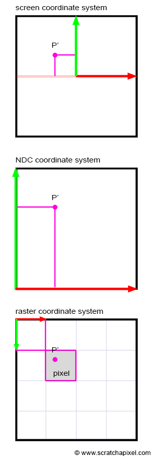
If the coordinates of P are real numbers (floats or doubles in programming), P's coordinates are also real numbers. If P's coordinates are within the canvas boundaries, then P' is visible. Otherwise, the point is not visible, and we can ignore it. If P' is visible, it should appear as a dot in the image. A dot in a digital image is a pixel. Note that pixels are also 2D points, but their coordinates are integers, and the coordinate system to which these coordinates refer is located in the upper-left corner of the image. Its x-axis points to the right (when the world coordinate system's x-axis points to the right), and its y-axis points downwards (Figure 11). This coordinate system in computer graphics is called the raster coordinate system. A pixel in this coordinate system is one unit long in both x and y. We need to convert P's coordinates, defined with respect to the image or screen coordinate system, into pixel coordinates (the position of P' in the image in terms of pixel coordinates). This is another change in the coordinate system; we say that we need to go from screen space to raster space. How do we do that?
The first thing we will do is remap P's coordinates to the range [0,1]. This is mathematically straightforward. Since we know the dimensions of the canvas, all we need to do is apply the following formulas:
$$ \begin{array}{l} P'_{normalized}.x = \dfrac{P'.x + \text{width} / 2}{\text{width}}\\ P'_{normalized}.y = \dfrac{P'.y + \text{height} / 2}{\text{height}} \end{array} $$Because the coordinates of the projected point P' are now in the range [0,1], we say that the coordinates are normalized. For this reason, we also call the coordinate system in which the points are defined after normalization the NDC coordinate system or NDC space. NDC stands for Normalized Device Coordinates. The NDC coordinate system's origin is situated in the lower-left corner of the canvas. Note that the coordinates are still real numbers at this point, only they are now in the range [0,1].
The last step is simple. We need to multiply the projected point's x- and y-coordinates in NDC space by the actual image pixel width and image pixel height, respectively. This is a simple remapping of the range [0,1] to the range [0, Pixel Width] for the x-coordinate and [0, Pixel Height] for the y-coordinate, respectively. Since the pixel coordinates need to be integers, we need to round off the resulting numbers to the smallest following integer value (to do that, we will use the mathematical floor function; it rounds off a real number to its nearest lower integer). After this final step, P's coordinates are defined in raster space:
$$ \begin{array}{l} P'_{raster}.x = \lfloor{ P'_{normalized}.x \times \text{ Pixel Width} }\rfloor\\ P'_{raster}.y = \lfloor{ (1 - P'_{normalized}.y) \times \text{Pixel Height} }\rfloor \end{array} $$In mathematics, \(\lfloor{a}\rfloor\) denotes the floor function. Pixel width and pixel height are the actual dimensions of the image in pixels. However, there is a small detail that we need to take care of. The y-axis in the NDC coordinate system points up, while in the raster coordinate system, the y-axis points down. Thus, to go from one coordinate system to the other, the y-coordinate of P' also needs to be inverted. We can easily account for this by making a small modification to the above equations:
$$ \begin{array}{l} P'_{raster}.x = \lfloor{ P'_{normalized}.x \times \text{ Pixel Width} }\rfloor\\ P'_{raster}.y = \lfloor{ (1 - P'_{normalized}.y) \times \text{Pixel Height} }\rfloor \end{array} $$In OpenGL, the conversion from NDC space to raster space is called the viewport transform. The canvas in this lesson is generally called the viewport in CG. However, the term 'viewport' means different things to different people. To some, it designates the "normalized window" of the NDC space. To others, it represents the window of pixels on the screen in which the final image is displayed.
Done! You have converted a point P defined in world space into a visible point in the image, whose pixel coordinates you have computed using a series of conversion operations:
-
World space to camera space.
-
Camera space to screen space.
-
Screen space to NDC space.
-
NDC space to raster space.
Summary
This chapter has outlined fundamental processes in 3D graphics rendering, emphasizing the transformation of points across various coordinate systems. Here’s a summary of what we've learned:
-
Points in a 3D scene are initially defined with respect to the world coordinate system.
-
A 4x4 matrix can be viewed as a "local" coordinate system.
-
We discussed how to convert points from the world coordinate system to any local coordinate system:
-
If we know the local-to-world matrix, we can transform the world coordinates of a point using the inverse of this matrix (the world-to-local matrix).
-
-
4x4 matrices are also crucial in transforming cameras, allowing the conversion of points from world space to camera space.
-
Computing the coordinates of a point from camera space onto the canvas can be achieved using perspective projection (camera space to image space). This method requires a simple division of the point's x- and y-coordinates by its z-coordinate. Before projecting the point onto the canvas, it is necessary to convert the point from world space to camera space. The result is a 2D point defined in image space (the z-coordinate is irrelevant).
-
We then convert the 2D point in image space to Normalized Device Coordinate (NDC) space. In NDC space (image space to NDC space), the point's coordinates are remapped to the range [0,1].
-
Finally, we transform the 2D point in NDC space to raster space. This requires multiplying the NDC point's x- and y-coordinates by the image width and height (in pixels). Since pixel coordinates must be integers, they are rounded to the nearest lower integer when converting from NDC space to raster space. In the NDC coordinate system, the y-axis is located in the lower-left corner of the image and points upward. In raster space, the y-axis is in the upper-left corner of the image and points downward. Thus, the y-coordinates need to be inverted when converting from NDC to raster space.
-
World Space
-
The space in which points are originally defined in the 3D scene. Coordinates of points in world space are defined with respect to the world Cartesian coordinate system.
-
-
Camera Space
-
The space in which points are defined with respect to the camera coordinate system. To convert points from world to camera space, we need to multiply points in world space by the inverse of the camera-to-world matrix. By default, the camera is located at the origin and is oriented along the world coordinate system's negative z-axis. Once the points are in camera space, they can be projected onto the canvas using perspective projection.
-
-
Screen Space
-
In this space, points are in 2D; they lie on the image plane. Because the plane is infinite, the canvas defines the region of this plane on which the scene can be drawn. The canvas size is arbitrary and defines "how much" of the scene we see. The image or screen coordinate system marks the center of the canvas (and the image plane's). If a point on the image plane is outside the boundaries of the canvas, it is not visible. Otherwise, the point is visible on the screen.
-
-
NDC Space
-
2D points lying in the image plane and contained within the boundaries of the canvas are then converted to Normalized Device Coordinate (NDC) space. The principle is to normalize the point's coordinates, in other words, to remap them to the range [0,1]. Note that NDC coordinates are still real numbers.
-
-
Raster Space
-
Finally, 2D points in NDC space are converted to 2D pixel coordinates. To do this, we multiply the normalized points' x and y coordinates by the image width and height in pixels. Going from NDC to raster space also requires the y-coordinate of the point to be inverted. Final coordinates need to be rounded to the nearest following integers since pixel coordinates are integers.
-
Code
The function converts a point from 3D world coordinates to 2D pixel coordinates and returns false if the point is not visible on the canvas. This implementation is quite naive; efficiency was not the primary concern when it was written. Instead, we structured it to ensure that every step is visible and contained within a single function.
bool computePixelCoordinates(
    const Vec3f &pWorld,
    const Matrix44f &cameraToWorld,
    const float &canvasWidth,
    const float &canvasHeight,
    const int &imageWidth,
    const int &imageHeight,
    Vec2i &pRaster)
{
    // First, transform the 3D point from world space to camera space.
    // It is inefficient to compute the inverse of the cameraToWorld matrix
    // in this function; it should be computed just once outside the function,
    // and the worldToCamera matrix should be passed in instead.
    Vec3f pCamera;
    Matrix44f worldToCamera = cameraToWorld.inverse();
    worldToCamera.multVecMatrix(pWorld, pCamera);

    // Coordinates of the point on the canvas, using perspective projection.
    Vec2f pScreen;
    pScreen.x = pCamera.x / -pCamera.z;
    pScreen.y = pCamera.y / -pCamera.z;

    // If the absolute values of the x- or y-coordinates exceed the canvas width
    // or height, respectively, the point is not visible.
    if (std::abs(pScreen.x) > canvasWidth || std::abs(pScreen.y) > canvasHeight)
        return false;

    // Normalize the coordinates to range [0,1].
    Vec2f pNDC;
    pNDC.x = (pScreen.x + canvasWidth / 2) / canvasWidth;
    pNDC.y = (pScreen.y + canvasHeight / 2) / canvasHeight;

    // Convert to pixel coordinates and invert the y-coordinate.
    pRaster.x = std::floor(pNDC.x * imageWidth);
    pRaster.y = std::floor((1 - pNDC.y) * imageHeight);

    return true;
}

int main(...)
{
    ...
    Matrix44f cameraToWorld(...);
    Vec3f pWorld(...);
    float canvasWidth = 2, canvasHeight = 2;
    uint32_t imageWidth = 512, imageHeight = 512;

    // Determine the 2D pixel coordinates of pWorld in the image if the point is visible.
    Vec2i pRaster;
    if (computePixelCoordinates(pWorld, cameraToWorld, canvasWidth, canvasHeight, imageWidth, imageHeight, pRaster)) {
        std::cerr << "Pixel coordinates: " << pRaster << std::endl;
    }
    else {
        std::cerr << pWorld << " is not visible" << std::endl;
    }
    ...

    return 0;
}
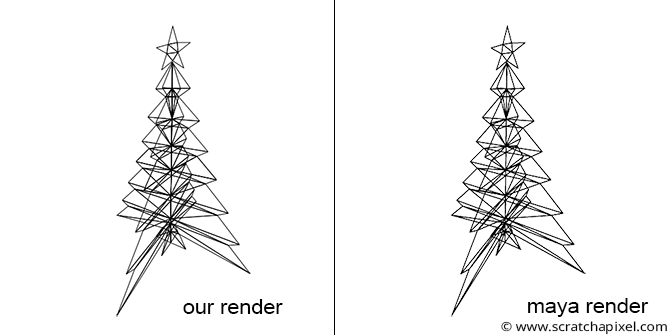
We will use a similar function in our example program (refer to the source code chapter). To demonstrate the technique, we created a simple object in Maya (a tree with a star on top) and rendered an image of that tree from a specified camera in Maya (see the image below). To simplify the exercise, we triangulated the geometry. We then stored a description of that geometry and the Maya camera 4x4 transform matrix (the camera-to-world matrix) in our program.
To create an image of that object, we need to:
-
Loop over each triangle that makes up the geometry.
-
Extract the vertices that form the current triangle from the vertex list.
-
Convert these vertices' world coordinates to 2D pixel coordinates.
-
Draw lines connecting the resulting 2D points to render the triangle as viewed from the camera (we trace a line from the first point to the second, from the second to the third, and then from the third back to the first point).
We then store the resulting lines in an SVG file. The SVG format is designed for creating images using simple geometric shapes, such as lines, rectangles, and circles, which are described in XML. Here is an example of how we define a line in SVG:
<line x1="0" y1="0" x2="200" y2="200" style="stroke:rgb(255,0,0);stroke-width:2" />
SVG files can be read and displayed as images by most internet browsers. Storing the result of our programs in SVG is convenient. Rather than rendering these shapes ourselves, we store their description in an SVG file and let other applications render the final image for us.
The complete source code of this program can be found in the source code chapter. Finally, here is the result of our program (left) compared to a render of the same geometry from the same camera in Maya (right). As expected, the visual results are identical (you can read the SVG file produced by the program in any internet browser).
Suppose you wish to reproduce this result in Maya. In that case, you will need to import the geometry (which we provide in the next chapter as an OBJ file), create a camera, set its angle of view to 90 degrees (we will explain why in the next lesson), and make the film gate square (by setting the vertical and horizontal film gate parameters to 1). Set the render resolution to 512x512 and render from Maya. You should then export the camera's transformation matrix using, for example, the following MEL command:
getAttr camera1.worldMatrix;
Set the camera-to-world matrix in our program with the result of this command (the 16 coefficients of the matrix). Compile the source code and run the program. The output exported to the SVG file should match Maya's render.
What Else?
This chapter contains a wealth of information. Most resources devoted to the perspective process emphasize the perspective transformation but often overlook essential steps like the world-to-camera transformation or the conversion of screen coordinates to raster coordinates. Our goal is to enable you to produce an actual result by the end of this lesson, one that could match a render from a professional 3D application such as Maya. We aim to give you a comprehensive overview of the process from start to finish. However, dealing with cameras is slightly more complex than described here. For example, if you have previously used a 3D program, you might be aware that the camera transform is not the only adjustable parameter affecting the camera's view. You can also alter the focal length, for instance. We have not yet explained how changing the focal length impacts the conversion process. Additionally, the near and far clipping planes associated with cameras influence the perspective projection process, notably affecting both the perspective and orthographic projection matrices. In this lesson, we assumed the canvas was positioned one unit away from the camera's coordinate system. However, this is not always the case, and it can be adjusted via the near-clipping plane. How do we compute pixel coordinates when the distance between the camera coordinate system's origin and the canvas differs from one unit? These unanswered questions will be addressed in our next lesson, which is devoted to 3D viewing.
Exercises
-
Change the dimensions of the canvas in the program (
canvasWidthandcanvasHeightparameters). Keep the values of these two parameters equal. What happens when the values decrease? What occurs when they increase?