Projection Matrices: What You Need to Know First
Reading time: 17 mins.Essential Preknowledge
To begin our exploration of constructing a simple perspective projection matrix, it's crucial to revisit the foundational techniques on which projection matrices are based.
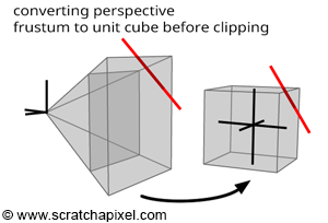
Transforming the Perspective Frustum into a Canonical Volume
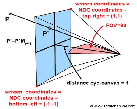
When a point P is transformed by a straightforward perspective projection matrix, it yields a point P', characterized by:
-
The x'- and y'-coordinates represent P's location on the image plane, both situated in Normalized Device Coordinates (NDC) space. As outlined earlier, the perspective projection matrix maps the coordinates of a 3D point to its "2D" screen position within NDC space (spanning [-1,1]). Typically, this matrix ensures that points within the camera's view (inside the frustum) map to the range [-1,1], regardless of the canvas shape - these coordinates are in NDC, not screen space.
-
Beyond mapping the 3D point to 2D coordinates, it's also necessary to adjust its z-coordinate. Unlike in our prior discussion on rasterization where z' remapping wasn't addressed, GPUs do remap the z-coordinate of P' into a range of [0,1] or [-1,1], depending on the graphics API used. For points on the near-clipping plane, z' maps to 0 (or -1), and for points on the far-clipping plane, z' maps to 1.
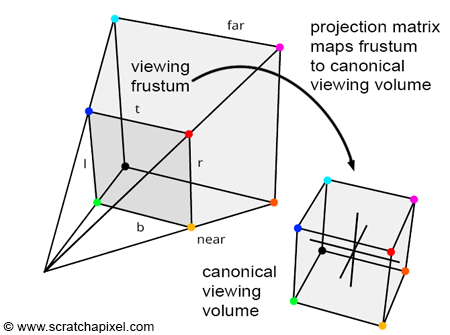
The remapping of P's x- and y-coordinates, as well as its z-coordinate to the ranges [-1,1] and [0,1] (or [-1,1]), signifies that the projection matrix transformation alters the viewing frustum's volume into a 2x2x1 (or 2x2x2) dimensional cube, commonly known as the unit cube or canonical view volume. This transformation can be viewed as normalizing the viewing frustum. While initially not cube-shaped but rather a truncated pyramid, the frustum is effectively "warped" into a cube through this process. This operation, performed by the projection matrix, is a pivotal concept in Computer Graphics (CG). It simplifies further operations on points by converting the viewing frustum, defined by the near and far clipping planes and screen dimensions, into a much more manageable geometric shape. Remembering that a projection matrix, in CG context, transforms the space delineated by the viewing frustum into a unit cube is vital.
Understanding Clipping
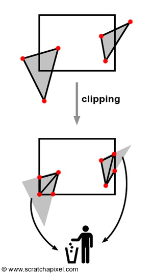
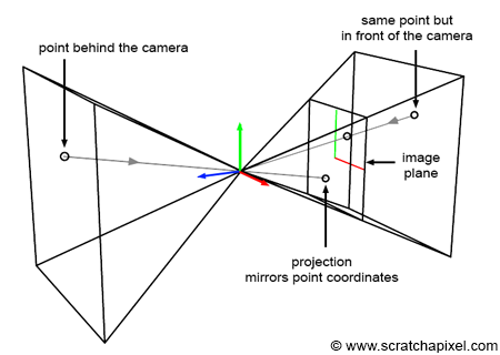
Clipping is the process of trimming geometry that intersects with the edges of the viewing frustum. Essentially, it ensures that only the portions of geometry within the frustum are retained while discarding those outside and hence not visible to the camera (as seen in figure 3). Although clipping might seem primarily like an optimization to discard unseen scene parts, its critical role is in managing how objects, regardless of their position relative to the camera, are projected. Consider a point behind the observer, for example, with coordinates (2, 5, 10). Applying perspective projection rules yields:
$$ \begin{array}{l} x' = \dfrac{2}{-10} = -0.2,\\ y' = \dfrac{5}{-10} = -0.5, \end{array} $$This shows that, despite the point's valid projected coordinates, it is mirrored on the canvas in both directions. While the original x- and y-coordinates are positive, their projections become negative in screen space (as depicted in figure 4).
A future discussion will introduce the Cohen-Sutherland algorithm, a prevalent method for clipping, within the context of advanced rasterization. However, our next chapter will delve deeper into clipping and clip space concepts.
-
The transformation from the complex shape of a viewing frustum (a truncated pyramid) to a simple box (canonical view volume) facilitates operations like clipping.
-
Defining geometry within this canonical view volume simplifies the conversion of 3D coordinates to 2D coordinates on the image plane.
This framework is designed to mimic the pinhole camera model, characterized by near and far clipping planes and an angle of view (detailed in the lesson on the pinhole camera model). The angle of view is particularly important when mapping points from screen space to NDC space.
Projecting Points onto the Screen
Before exploring the construction of a perspective matrix, it's worth revisiting the projection of 3D points onto the screen. This method, fully explained in Computing the Pixel Coordinates of a 3D Point, involves initially transforming 3D points into the camera's coordinate system. Here, the camera's position is the origin, with the x- and y-axes parallel to the image plane and the z-axis perpendicular. Our setup positions the image plane one unit from the camera's origin to simplify demonstrations, although arbitrary distances can be accommodated in more complex models.
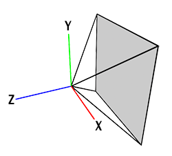
Scratchapixel adopts a right-hand coordinate system, common among many commercial applications like Maya. This setup means the camera points in the direction opposite the z-axis, ensuring that visible points have a negative z-component when defined in the camera coordinate system. This convention is crucial for projecting points accurately onto the image plane.
To project a point P onto the canvas and find its corresponding point P', draw a line from P through the eye to the image plane.
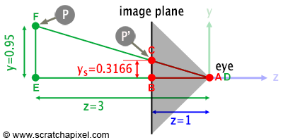
In Figure 6, triangles \(\Delta ABC\) and \(\Delta DEF\) are similar, meaning they share the same shape but differ in size. This similarity implies a constant ratio between their sides, leading to the equation:
$$\dfrac{BC} {EF} = \dfrac{AB} {DE}.$$To find BC, the position of P' on the image plane, we use:
$$BC = \dfrac{AB * EF} {DE}.$$With B on the image plane and one unit from A (AB = 1), we derive:
$$BC = \dfrac{(AB=1) * EF} {DE} = \dfrac{EF} {DE}.$$This yields the x- and y-coordinates of P' through division of P's coordinates by its z-coordinate:
$$ \begin{array}{l} P'_x=\dfrac{P_x}{-P_z},\\ P'_y=\ dfrac{P_y}{-P_z}. \end{array} $$Here, division by \(-P_z\) accounts for the camera system's convention where visible points have a negative z-component. This simplifies computing P', the projection of P on the image plane, with Figure 6 illustrating the y-coordinate projection. Rotating this figure ninety degrees and substituting the y-axis with the x-axis provides a top view for projecting P's x-coordinate.
Homogeneous Coordinates

Though perspective projection might seem straightforward, the complexity arises when we seek to encapsulate this process within a matrix, allowing point projection onto the image plane through basic point-matrix multiplication. Let's recap our understanding of this process.
Recall from our discussions in the lesson on Geometry that two matrices can be multiplied if the number of columns in the left matrix equals the number of rows in the right matrix:
$$ \begin{array}{l} {\color{red} {\text{no:}}} & [n \: m] * [q \: n] \\ {\color{green} {\text{yes:}}} & [m \: n] * [n \: q] \\ \end{array} $$A point is typically represented as a one-row matrix. However, such a 1x3 matrix cannot be directly multiplied by a 4x4 matrix, which is standard in CG for encoding transformations including rotation, scale, and translation. The solution is to represent points not with three, but with four coordinates, adopting homogeneous coordinates in a 1x4 matrix form. The fourth coordinate, w, is set to 1 when converting from Cartesian to homogeneous coordinates, making \(P_c\) (a point in Cartesian coordinates) and \(P_h\) (in homogeneous coordinates) interchangeable as long as \(w = 1\). If \(w \neq 1\), it's necessary to normalize the point by dividing its coordinates [x y z w] by \(w\) to revert \(w\) to 1 for Cartesian usage.
$$ \begin{array}{l} [x \: y \: z] \neq [x \: y \: z \: w=1.2] \\ x=\dfrac{x}{w}, \: y=\dfrac{y}{w}, \: z=\dfrac{z}{w}, \: w=\dfrac{w}{w}=1 \\ {[x \: y \: z] = [x \: y \: z \: w = 1]} \end{array} $$A more formal definition states that the point with homogeneous coordinates [x, y, z, w] corresponds to the three-dimensional Cartesian point [x/w, y/w, z/w].
A typical transformation matrix is structured as follows, where the [3x3] inner matrix (green) represents rotation and scale, and the bottom row coefficients (red) handle translation:
$$ \begin{bmatrix} \color{green}{m_{00}} & \color{green}{m_{01}} & \color{green}{m_{02}} & \color{blue}{0}\\ \color{green}{m_{10}} & \color{green}{m_{11}} & \color{green}{m_{12}} & \color{blue}{0}\\ \color{green}{m_{20}} & \color{green}{m_{21}} & \color{green}{m_{22}} & \color{blue}{0}\\ \color{red}{T_x} & \color{red}{T_y} & \color{red}{T_z} & \color{blue}{1}\\ \end{bmatrix} $$In practice, we treat 3D points as if they had homogeneous coordinates by implicitly setting their fourth coordinate, w, to 1. This allows for efficient multiplication by 4x4 matrices without explicitly defining points with four coordinates, conserving memory. To convert back to Cartesian coordinates after transformation, the transformed coordinates \(x', y', z'\) are divided by \(w'\), although in the case of affine transformations, where the fourth row is always \([0, 0, 0, 1]\), this step is often unnecessary as \(w'\) remains 1.
Remember that 4x4 transformation matrices are considered affine. These matrices have two key attributes:
-
Collinearity Preservation: Points on a line remain aligned post-transformation.
-
Distance Ratios Preservation: The midpoint of a segment maintains its position relative to the segment's ends after transformation.
This distinction is crucial because, unlike affine transformations, projective transformations retain collinearity but not the ratios of distances. This aspect was highlighted previously, noting that perspective projection keeps lines intact while altering distances between points.
In the context of transforming 3D points, we effectively treat these points as though they have homogeneous coordinates. This approach involves an "implicit" assumption that these 3D points include a fourth coordinate set to 1. It's important to recognize that a 3D point defined by {x, y, z} and a point in homogeneous coordinates {x, y, z, w} are equivalent as long as w equals 1. This allows us to express a 3D point in homogeneous coordinates as:
$$P = \{x, y, z, w = 1\}.$$Keep in mind, when a "3D" point is subjected to multiplication by a 4x4 matrix, it is considered (implicitly, if not explicitly defined with four coordinates in certain software) a point in homogeneous coordinates with a w-coordinate of 1. The reason for not "explicitly" defining points with four coordinates in programming is to conserve memory, avoiding the unnecessary storage of a constantly 1-valued coordinate. Proceeding to multiply this 1x4 matrix representation (our point) by a 4x4 transformation matrix, we expect to obtain another point in homogeneous coordinates. To revert this point back to 3D, we must divide the transformed coordinates {x', y', z'} by w. However, the fourth row of a 4x4 transformation matrix being consistently set to \(\color{blue}{{0, 0, 0, 1}}\) ensures the w-coordinate of the transformed point, \(\color{purple}{w'}\), remains always 1. This outcome arises from the multiplication mechanism:
$$ \begin{bmatrix} x' & y' & z' & w' \end{bmatrix} = \begin{bmatrix} x & y & z & w = 1 \end{bmatrix} * \begin{bmatrix} \color{green}{m_{00}} & \color{green}{m_{01}} & \color{green}{m_{02}} & \color{blue}{0}\\ \color{green}{m_{10}} & \color{green}{m_{11}} & \color{green}{m_{12}} & \color{blue}{0}\\ \color{green}{m_{20}} & \color{green}{m_{21}} & \color{green}{m_{22}} & \color{blue}{0}\\ \color{red}{T_x} & \color{red}{T_y} & \color{red}{T_z} & \color{blue}{1}\\ \end{bmatrix} $$ $$ \begin{array}{l} x' = x * m_{00} + y * m_{10} + z * m_{20} + (w = 1) * T_x,\\ y' = x * m_{01} + y * m_{11} + z * m_{21} + (w = 1) * T_y,\\ z' = x * m_{02} + y * m_{12} + z * m_{22} + (w = 1) * T_z,\\ \color{purple}{w' = x * 0 + y * 0 + z * 0 + (w = 1) * 1 = 1}.\\ \end{array} $$No matter the values within the 3x3 matrix or the translation coefficients, \(\color{purple}{w'}\) consistently equals 1. This is because \(\color{purple}{w'}\) is derived from w set to 1 and the matrix's fourth column coefficients, which are invariably \(\color{blue}{{0, 0, 0, 1}}\). These coefficients are static, unchanging and thus define the matrix as transformational rather than projective. Consequently, there's no need to convert the x', y', and z' coordinates back to Cartesian by dividing them by \(\color{purple}{w'}\), since \(\color{purple}{w'}\) is always 1.
A 3D Cartesian point P, when transformed to homogeneous coordinates {x, y, z, w = 1} and multiplied by a 4x4 affine transformation matrix, invariably results in a point P' in homogeneous coordinates with a w-coordinate \(\color{purple}{w'}\) perpetually at 1. Therefore, transforming the point P' back to 3D Cartesian coordinates {x'/w', y'/w', z'/w'} does not necessitate an explicit normalization by \(\color{purple}{w'}\), simplifying the conversion process.
Technical implementation for multiplying a point by a 4x4 matrix can be illustrated through three versions of a function, each progressively simplified based on the assumption of homogeneous coordinates:
Version 1 of the function, designed for points explicitly defined in homogeneous coordinates (Vec4), incorporates the w-coordinate in calculations:
template<typename S>
void multVecMatrix(const Vec4<S> &src, Vec3<S> &dst) const
{
    S a, b, c, w;

    // Note: src.w is assumed to be 1
    a = src.x * x[0][0] + src.y * x[1][0] + src.z * x[2][0] + src.w * x[3][0];
    b = src.x * x[0][1] + src.y * x[1][1] + src.z * x[2][1] + src.w * x[3][1];
    c = src.x * x[0][2] + src.y * x[1][2] + src.z * x[2][2] + src.w * x[3][2];
    w = src.x * x[0][3] + src.y * x[1][3] + src.z * x[2][3] + src.w * x[3][3];

    dst.x = a / w;
    dst.y = b / w;
    dst.z = c / w;
}
This formulation acknowledges that the source point possesses four coordinates, facilitating multiplication by a 4x4 matrix. Given the homogeneous coordinate system's nature, where src.w is always 1, this version can be optimized.
Version 2 simplifies the process by implicitly treating the source point as having a w-coordinate of 1, thus not needing explicit definition. This version adapts to points represented as Vec3 for efficiency:
template<typename S>
void multVecMatrix(const Vec3<S> &src, Vec3<S> &dst) const
{
    S a, b, c, w;

    // Implicitly treating src.w as 1
    a = src.x * x[0][0] + src.y * x[1][0] + src.z * x[2][0] + x[3][0];
    b = src.x * x[0][1] + src.y * x[1][1] + src.z * x[2][1] + x[3][1];
    c = src.x * x[0][2] + src.y * x[1][2] + src.z * x[2][2] + x[3][2];
    w = src.x * x[0][3] + src.y * x[1][3] + src.z * x[2][3] + x[3][3];

    dst.x = a / w;
    dst.y = b / w;
    dst.z = c / w;
}
Given that affine transformation matrices guarantee w remains 1, further optimization is possible, eliminating the need for division by w.
Version 3 represents the most streamlined approach, directly applicable for affine transformations, where the computation of w and subsequent division is unnecessary:
template<typename S>
void multVecMatrix(const Vec3<S> &src, Vec3<S> &dst) const
{
    S a, b, c;

    // Direct calculation without explicit w
    a = src.x * x[0][0] + src.y * x[1][0] + src.z * x[2][0] + x[3][0];
    b = src.x * x[0][1] + src.y * x[1][1] + src.z * x[2][1] + x[3][1];
    c = src.x * x[0][2] + src.y * x[1][2] + src.z * x[2][2] + x[3][2];

    // Affine transformation implies w = 1; no division required
    dst.x = a;
    dst.y = b;
    dst.z = c;
}
This final version is commonly employed for transforming points with affine matrices, emphasizing efficiency by leveraging the uniform nature of w-coordinate in affine transformations.
Why have we delved into such a detailed discussion? Primarily, it's to deepen our understanding of homogeneous coordinates, a cornerstone concept in computer graphics (CG). In CG, we predominantly engage with two kinds of matrices: 4x4 affine transformation matrices and 4x4 projection matrices. As we've explored, affine transformation matrices maintain the \(w\)-coordinate of transformed points at 1. However, projection matrices, which are the focus of this lesson, operate differently. When a point undergoes transformation via a projection matrix, its \(x'\), \(y'\), and \(z'\) coordinates must be normalized—a step that is not required with affine transformation matrices.
Affine Transform Matrix:
-
Input 3D point is implicitly converted to homogeneous coordinates {x, y, z, w = 1}.
-
The elements \(m_{30}, m_{31}, m_{32}\), and \(m_{33}\) are always equal to {0, 0, 0, 1} respectively.
-
\(w'\) is always equal to 1, eliminating the need to compute \(w'\):
$$ \begin{array}{l} w' &=& x * (m_{30} = 0) + \\ && y * (m_{31}= 0) + \\ && z * (m_{32} = 0) + \\ && (w = 1) * 1 \\ & = & 1 \end{array} $$ -
Normalization is never needed, allowing direct use of transformed coordinates:
$$ \begin{array}{l} P'_H = \{x', y', z', w'=1\} \\ P'_C = \{x', y', z'\} \end{array} $$
Projection Matrix (perspective or orthographic):
-
Input 3D point is implicitly converted to homogeneous coordinates {x, y, z, w = 1}, similar to the affine transform matrix.
-
The elements \(m_{30}, m_{31}, m_{32}\), and \(m_{33}\) vary and are specific to the type of projection matrix, which will be detailed further.
-
\(w'\) could differ from 1 and must be explicitly computed:
$$ \begin{array}{l} w' & = & x * (m_{30} != 0) + \\ && y * (m_{31} != 0) + \\ && z * (m_{32} != 0) + \\ && (w = 1) * (m_{33} != 1) \\ & != & 1 \end{array} $$ -
Normalization of the point is necessary if \(w' \neq 1\), converting the homogeneous coordinates back to Cartesian:
$$ \begin{array}{l} P'_H = \{x', y', z', w' \neq 1\} \\ P'_C = \{x'/w', y'/w', z'/w'\} \end{array} $$
Understanding the distinction between affine transformation matrices and projection matrices is crucial. When a point is multiplied by a projection matrix, it necessitates a specific version of the point-matrix multiplication function. This version must explicitly calculate \(w\) and normalize the coordinates of the transformed point, akin to this approach (version 2):
template<typename S>
void multVecMatrix(const Vec3<S> &src, Vec3<S> &dst) const
{
    S a, b, c, w;

    // Implicitly treating src.w as always 1
    a = src.x * x[0][0] + src.y * x[1][0] + src.z * x[2][0] + x[3][0];
    b = src.x * x[0][1] + src.y * x[1][1] + src.z * x[2][1] + x[3][1];
    c = src.x * x[0][2] + src.y * x[1][2] + src.z * x[2][2] + x[3][2];
    w = src.x * x[0][3] + src.y * x[1][3] + src.z * x[2][3] + x[3][3];

    dst.x = a / w;
    dst.y = b / w;
    dst.z = c / w;
}
Skipping this function with projection matrices leads to inaccurate outcomes. However, for efficiency, this method is not preferred when working with affine transformation matrices, where \(w'\) doesn't require calculation and the coordinates don't need normalization. The usual practice might involve having two separate functions for each matrix type, though this is seldom implemented. Programmers typically opt for a more general approach, such as this, which circumvents unnecessary division for \(w = 1\):
template<typename S>
void multVecMatrix(const Vec3<S> &src, Vec3<S> &dst) const
{
    S a, b, c, w;

    // Assuming src.w is always 1 for simplicity
    a = src.x * x[0][0] + src.y * x[1][0] + src.z * x[2][0] + x[3][0];
    b = src.x * x[0][1] + src.y * x[1][1] + src.z * x[2][1] + x[3][1];
    c = src.x * x[0][2] + src.y * x[1][2] + src.z * x[2][2] + x[3][2];
    w = src.x * x[0][3] + src.y * x[1][3] + src.z * x[2][3] + x[3][3];

    if (w != 1) {
        dst.x = a / w;
        dst.y = b / w;
        dst.z = c / w;
    }
    else {
        dst.x = a;
        dst.y = b;
        dst.z = c;
    }
}
This adaptable code caters to both affine transformations and projection matrices. The extensive discussion on homogeneous coordinates highlights the normalization step's pivotal role in projection matrix operations, a topic we'll delve deeper into in the forthcoming chapter.