Möller-Trumbore algorithm
Reading time: 24 mins.Möller-Trumbore algorithm
The Möller-Trumbore algorithm is a fast ray-triangle intersection algorithm that was introduced in 1997 by Tomas Möller and Ben Trumbore in a paper titled "Fast, Minimum Storage Ray/Triangle Intersection". It is still considered today a fast algorithm that is often used in benchmarks to compare the performances of other methods. However, a fair comparison of ray-triangle intersection algorithms is difficult because speed can depend on many factors, such as how algorithms are implemented, the type of test scene used, whether values are precomputed, etc.
The Möller-Trumbore algorithm takes advantage of the parameterization of P, the intersection point in barycentric coordinates (which we discussed in the previous chapter). We learned in the previous chapter to calculate P, the intersection point, using the following equation:
$$P = wA + uB + vC$$We also learned that \(w=1-u-v\); thus, we can write:
$$P = (1 - u - v)A + uB + vC$$Note that the paper by Möller-Trumbore uses the convention \( P = (1 - u - v)A + uB + vC \) instead of \( P = uA + vB + (1 - u - v)C \), which we've been using in the chapter on barycentric coordinates. As I mentioned in that chapter, the way you pair the barycentric coordinates and the vertices is entirely up to you, as long as the edges you use in the calculation of \( u \), \( v \), and \( w \) are adapted to the pairing convention you've chosen.
As explained in that chapter, the pairing convention chosen by Möller-Trumbore comes from the fact that you can write \( P = A + uAB + vAC \), which can be interpreted as: "start from \( A \), the origin, and then move along the line \( AB \) by \( u \), as well as along the line \( AC \) by \( v \), to find \( P \)." If you expand the vectors \( AB \) and \( AC \) as \( B - A \) and \( C - A \), respectively, you get:
$$ \begin{array}{l} P = A + u(B - A) + v(C - A) \\ P = A + uB - uA + vC - vA \\ P = (1 - u - v)A + uB + vC \end{array} $$This is the formulation used by Möller-Trumbore, and this derivation explains why it is a convention commonly used in research papers and books, as opposed to the \( uA + vB + wC \) formulation that we've used in the chapter on barycentric coordinates, which is also frequently found in code.
I will stick to the convention used in the paper so that the lesson and the paper remain consistent. Bottom line: stay aware of this pairing issue. Let's move on with the rest of the demonstration.
If we develop, we get (equation 1):
$$ \begin{equation} P=A - uA - vA + uB + vC = A + u(B - A) + v(C - A) \end{equation} $$Note that \( (B - A) \) and \( (C - A) \) are the edges \( AB \) and \( AC \) of the triangle \( \triangle ABC \). The intersection point \( P \) can also be written using the ray's parametric equation (Equation 2).
$$ \begin{equation} P=O+tD. \end{equation} $$Where \(t\) is the distance from the ray's origin to the intersection \(P\). If we replace \(P\) in equation 1 with the ray's equation, we get (equation 3):
$$ \begin{equation} \begin{array}{l} O+tD & = & A + u(B - A) + v(C - A)\\ O-A & = & -tD+u(B-A)+v(C-A) \end{array} \end{equation} $$On the right side of the equal sign, we have:
-
\( t \), \( u \), and \( v \) as three unknowns,
-
respectively multiplied by \( B - A \), \( C - A \), and \( D \), which are three known variables.
We can rearrange these terms and present equation 3 using the following notation (equation 4):
$$ \begin{equation} \begin{bmatrix} -D & (B-A) & (C-A) \end{bmatrix} \begin{bmatrix} t\\ u\\ v \end{bmatrix} =O-A \end{equation} $$The left side of the equation has been rearranged into a row-column vector multiplication (1x3*3x1). This is the simplest possible form of matrix multiplication. You take the first element of the row matrix \(-D\), \(B-A\), \(C-A\) and multiply it by the first element of the column vector (\(t\), \(u\), \(v\)). Then you add the raw matrix's second element multiplied by the column vector's second element. Then finally, add the third element of the raw matrix multiplied by the third element of the column vector (which gives you equation 3 again).
In equation 3, the term \(O-A\) on the left side of the equal sign is a vector. \(B-A\), \(C-A\), and \(D\) are vectors as well, and \(t\), \(u\), and \(v\) (unknown) are scalars (floats or doubles if you prefer to think in terms of programming). This equation is about vectors. It combines three vectors in quantities defined by \(t\), \(u\), and \(v\). It gives another vector as a result of this operation (be aware that in their paper, Möller and Trumbore use the term x-, y- and z-axis instead of \(t\), \(u\) and \(v\) when they explain the geometrical meaning of this equation).
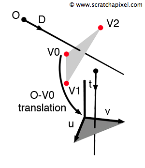
Let's say that \( P \) is where the ray intersects the triangle \( \triangle ABC \). You will (hopefully) agree that the Cartesian coordinates of point \( P \) (x, y, z) change as we move or rotate the triangle and the ray together. However, the barycentric coordinates of \( P \) are invariant. If the triangle is rotated, scaled, stretched, or translated, the coordinates \( u \) and \( v \), which define the position of \( P \) with respect to vertices \( A \), \( B \), and \( C \), will not change (see Figure 1).
The Möller-Trumbore algorithm takes advantage of this property. Instead of solving the ray-triangle intersection equation using the \(x\), \(y\), and \(z\) coordinates for the intersection point, it expresses the intersection point in terms of the triangle's barycentric coordinates \(u\) and \(v\). A point lying on the triangle (our intersection point, if it exists) can thus be expressed either in Cartesian coordinates \((x, y, z)\) or in barycentric coordinates \((u, v)\).
Finally, as we learned in the previous chapter, let's recall that the \(u\) and \(v\) coordinates of the point lying on the surface of a triangle can't be greater than one nor lower than 0. Their sum can't be greater than one either \(u + v <= 1\). They express coordinates of points defined inside a unit triangle (this is the triangle defined in \(u\), \(v\) space by the vertices (0, 0), (1, 0), (0, 1) as shown in Figure 1).
Let's summarize. What do we have so far? We have reinterpreted the three-dimensional \(x\), \(y\), \(z\) position of point \(P\) in terms of \(u\) and \(v\) barycentric coordinates, effectively moving from one parameter space to another: from xyz-space to uv-space. We have also learned that points defined in uv-space lie within a unit triangle.
Equation 3 (or 4, as they are identical) has three unknowns: \(u\), \(v\), and \(t\). Geometrically, we have already explained the meaning of \(u\) and \(v\). But what about \(t\)? Simply put, we will consider \(t\) as the third axis of the \(u\) and \(v\) coordinate system we just introduced. We now have a coordinate system defined by three axes: \(u\), \(v\), and \(t\).
Geometrically, let's explain what \(t\) represents. We know that \(t\) expresses the distance from the ray origin to \(P\), the intersection point. If you look at Figure 1, you can see that we have created a coordinate system that allows us to fully describe the position of the intersection point \(P\) in terms of barycentric coordinates and the distance from the ray origin to that point on the triangle.
Möller and Trumbore explain that the first part of Equation 4 (the term \( O - A \)) can be interpreted as a transformation that moves the triangle from its original world-space position to the origin (with the first vertex of the triangle coinciding with the origin). The other side of the equation transforms the intersection point from \(x, y, z\) space to "tuv-space," as explained above.
Cramer's Rule
What we need to do now is solve this equation, which has three unknowns: \(t\), \(u\), and \(v\). To solve Equation 4, Möller and Trumbore use a technique known in mathematics as Cramer's rule. Cramer's rule provides the solution to a system of linear equations in terms of determinants. It states that if the multiplication of a matrix \(M\) (a set of three numbers laid out horizontally) by a column vector \(X\) (three numbers laid out vertically) is equal to a column vector \(C\), then it is possible to find \(X_i\) (the \(i\)th element of the column vector \(X\)) by dividing the determinant of \(M_i\) by the determinant of \(M\). Here, \(M_i\) is the matrix formed by replacing the \(i\)th column of \(M\) with the column vector \(C\).
If you are unfamiliar with Cramer's rule, it is explained in the gray box below.
Imagine we need to solve for \(x\), \(y\), and \(z\) using the following set of linear equations:
$$ \begin{array}{l} 2x + 1y + 1z = 3 \\ 1x - 1y - 1z = 0 \\ 1x + 2y + 1z = 0 \end{array} $$We can rewrite these equations using a matrix representation, where the coefficients on the left become the elements of matrix \(M\), and the numbers on the right of the equal sign become the elements of matrix \(C\):
$$ M = \left[ \begin{array}{rrr} 2 & 1 & 1\\ 1 & -1 & -1\\ 1 & 2 & 1 \end{array} \right] $$ $$ C = \left[ \begin{array}{c} \color{red}{3}\\ \color{red}{0}\\ \color{red}{0} \end{array} \right] $$Thus, we can express this system of equations as:
$$ M \cdot \begin{bmatrix} x \\ y \\ z \end{bmatrix} = C $$By replacing the first column in \(M\) with \(C\), we create matrix \(M_x\):
$$ M_x = \left[ \begin{array}{rrr} \color{red}{3} & 1 & 1 \\ \color{red}{0} & -1 & -1 \\ \color{red}{0} & 2 & 1 \end{array} \right] $$Similarly, we can create \(M_y\) and \(M_z\):
$$ \begin{array}{l} M_y = \left[ \begin{array}{rrr} 2 & \color{red}{3} & 1 \\ 1 & \color{red}{0} & -1 \\ 1 & \color{red}{0} & 1 \end{array} \right] \\ M_z = \left[ \begin{array}{rrr} 2 & 1 & \color{red}{3} \\ 1 & -1 & \color{red}{0} \\ 1 & 2 & \color{red}{0} \end{array} \right] \end{array} $$Now, let's evaluate each determinant:
$$ \begin{array}{l} \left| M \right| = \left| \begin{array}{rrr} 2 & 1 & 1\\ 1 & -1 & -1\\ 1 & 2 & 1 \end{array} \right| = (-2) + (-1) + (2) - (-1) - (-4) - (1) = 3\\ \left| M_x \right| = \left| \begin{array}{rrr} \color{red}{3} & 1 & 1 \\ \color{red}{0} & -1 & -1 \\ \color{red}{0} & 2 & 1 \end{array} \right| = (-3) + (0) + (0) - (0) - (-6) - (0) = 3\\ \left| M_y \right| = \left| \begin{array}{rrr} 2 & \color{red}{3} & 1 \\ 1 & \color{red}{0} & -1 \\ 1 & \color{red}{0} & 1 \end{array} \right| = (0) + (-3) + (0) - (0) - (0) - (3) = -6\\ \left| M_z \right| = \left| \begin{array}{rrr} 2 & 1 & \color{red}{3} \\ 1 & -1 & \color{red}{0} \\ 1 & 2 & \color{red}{0} \end{array} \right| = (0) + (0) + (6) - (-3) - (0) - (0) = 9 \end{array} $$Remember that the determinant of a 3x3 matrix:
$$ \begin{vmatrix} a & b & c \\ d & e & f \\ g & h & i \end{vmatrix} $$has the value:
$$ (aei + bfg + cdh) - (ceg + bdi + afh). $$Cramer's rule states that \( x = \dfrac{M_x}{M} \), \( y = \dfrac{M_y}{M} \), and \( z = \dfrac{M_z}{M} \). Thus:
$$ \begin{array}{l} x = \dfrac{3}{3} = 1 \\ y = \dfrac{-6}{3} = -2 \\ z = \dfrac{9}{3} = 3 \end{array} $$In linear algebra, the determinant is denoted by two vertical bars, and it reads: \( \begin{vmatrix} I & J & K \end{vmatrix} \) is the determinant of the matrix having \( I \), \( J \), and \( K \) as its columns. Following the conventions used in the gray box above, you can now see that matrix \( M \) is \( [-D, B - A, C - A] \), \( X \) is \( [t, u, v] \), and \( C \) is \( O - A \) in our system of linear equations. We are interested in finding values for \( t \), \( u \), and \( v \). To understand how we apply Cramer's rule let's recap:
Cramer's rule states that for a system of linear equations \( MX = C \), where \( M \) is a matrix of coefficients, \( X \) is a vector of unknowns, and \( C \) is the result vector, the solution for each component \( X_i \) can be found by replacing the \( i \)-th column of the matrix \( M \) with the vector \( C \), then dividing the determinant of the resulting matrix by the determinant of \( M \).
In this case, the matrix \( M \) is \( [-D, B - A, C - A] \), and the right-hand side vector \( C \) is \( O - A \). So, the solution using Cramer's rule for the unknowns \( t \), \( u \), and \( v \) is:
$$ \begin{bmatrix} t \\ u \\ v \end{bmatrix} = \frac{1}{\text{det}(M)} \begin{bmatrix} \text{det}(M_t) \\ \text{det}(M_u) \\ \text{det}(M_v) \end{bmatrix} $$Where:
-
\( M_t \) is the matrix \( M \) with its first column replaced by \( O - A \),
-
\( M_u \) is the matrix \( M \) with its second column replaced by \( O - A \),
-
\( M_v \) is the matrix \( M \) with its third column replaced by \( O - A \).
Applying this technique to our problem gives (Equation 5):
$$ \left[ \begin{array}{r} t \\ u \\ v \end{array} \right] = \dfrac{1}{\left| \begin{array}{r} -D & E_1 & E_2 \end{array} \right|} \left[ \begin{array}{c} \left| \begin{array}{c} T & E_1 & E_2 \end{array} \right| \\ \left| \begin{array}{c} -D & T & E_2 \end{array} \right| \\ \left| \begin{array}{c} -D & E_1 & T \end{array} \right| \\ \end{array} \right], $$where, for brevity, we denote \( T = O - A \), \( E_1 = B - A \), and \( E_2 = C - A \). The equation for each unknown (\( t \), \( u \), and \( v \)) is expressed as the ratio of a determinant.
-
The determinant of \( M \) is written as \( \left| \begin{array}{r} -D & E_1 & E_2 \end{array} \right| \), where \( E_1 = B - A \) and \( E_2 = C - A \).
-
\( M_t \), \( M_u \), \( M_v \) are matrices where you replace the corresponding columns of \( M \) with \( T = O - A \). These are used to compute the determinants for \( t \), \( u \), and \( v \), respectively.
The next step is to find the values of these four determinants. In the lesson on Geometry, we explained that the determinant of a \(1 \times 3\) matrix \( \begin{vmatrix} A & B & C \end{vmatrix} \) can be calculated as follows (refer to the grey box below for more details on where these equations come from):
$$ |A \ B \ C| = -(A \times C) \cdot B = -(C \times B) \cdot A. $$The determinant of a \(3 \times 3\) matrix is a scalar triple product, which combines a cross product and a dot product. Therefore, we can rewrite Equation 5 as:
$$ \left[\begin{array}{r}t\\u\\v\end{array}\right] = \frac{1}{(D \times E_2) \cdot E_1} \begin{bmatrix} (T \times E_1) \cdot E_2\\ (D \times E_2) \cdot T\\ (T \times E_1) \cdot D \end{bmatrix} = \frac{1}{P \cdot E_1} \begin{bmatrix} Q \cdot E_2\\ P \cdot T\\ Q \cdot D \end{bmatrix}, $$where \( P = (D \times E_2) \) and \( Q = (T \times E_1) \).
It is now straightforward to find the values of \( t \), \( u \), and \( v \). We can obtain them using cross and dot products between known variables: the vertices of the triangle, the ray origin, and the ray direction. Very nice!
You may want to check the Wikipedia page on Triple Product for more information, but just in case you are in a hurry, let's recall some basic rules here that will help you understand the following equations:
-
Due to the cyclic permutation nature of the scalar triple product, all the following expressions evaluate to the same value:
$$ \mathbf{a} \cdot (\mathbf{b} \times \mathbf{c}) = \mathbf{b} \cdot (\mathbf{c} \times \mathbf{a}) = \mathbf{c} \cdot (\mathbf{a} \times \mathbf{b}) $$ -
Swapping the positions of the operators without re-ordering the operands leaves the triple product unchanged. This follows from the preceding property and the commutative property of the dot product:
$$ \mathbf{a} \cdot (\mathbf{b} \times \mathbf{c}) = (\mathbf{a} \times \mathbf{b}) \cdot \mathbf{c} $$ -
Swapping any two of the three operands negates the triple product. This follows from the anticommutativity property of the cross product:
$$ \mathbf{a} \cdot (\mathbf{b} \times \mathbf{c}) = -\mathbf{a} \cdot (\mathbf{c} \times \mathbf{b}) = -\mathbf{b} \cdot (\mathbf{a} \times \mathbf{c}) = -\mathbf{c} \cdot (\mathbf{b} \times \mathbf{a}) $$
Using these rules, when you encounter the determinant \( \left| -D \ T \ E_2 \right| \), you can express it as the triple product \((E_2 \times -D) \cdot T\). To eliminate the negative sign in front of \( T \), we can swap \( E_2 \) and \(-D\), resulting in \( (D \times E_2) \cdot T \). The other triple products can be derived using the rules provided above.
The scalar triple product can also be understood as the determinant of a \(3 \times 3\) matrix with the three vectors as either its rows or its columns:
$$ \mathbf{a} \cdot (\mathbf{b} \times \mathbf{c}) = \det \begin{bmatrix} a_1 & a_2 & a_3 \\ b_1 & b_2 & b_3 \\ c_1 & c_2 & c_3 \\ \end{bmatrix}. $$Implementation
Implementing the Möller-Trumbore algorithm is straightforward. The scalar triple product \( (A \times B) \cdot C \) is equivalent to \( A \cdot (B \times C) \). Therefore, the denominator \( (D \times E2) \cdot E1 \) in Equation 5 can be expressed as \( D \cdot (E1 \times E2) \). The cross product of \( E1 \) and \( E2 \) gives the normal of the triangle. If the dot product of the ray direction \( D \) and the triangle's normal is zero, then the triangle and the ray are parallel, resulting in no intersection.
It's important to consider whether to cull (discard) back-facing triangles (triangles facing away from the camera). If the triangle is front-facing, the determinant is positive; if it is back-facing, the determinant is negative. In the code, we first compute this determinant. There is no intersection if the determinant is negative and back-face culling is enabled, or if the determinant is close to zero. If the triangle is double-sided (not culled), we still need to check whether the determinant is close to zero, which requires a signed value comparison.
bool rayTriangleIntersect(
    const Vec3f &orig, const Vec3f &dir,
    const Vec3f &v0, const Vec3f &v1, const Vec3f &v2,
    float &t, float &u, float &v)
{
    Vec3f v0v1 = v1 - v0;
    Vec3f v0v2 = v2 - v0;
    Vec3f pvec = dir.crossProduct(v0v2);
    float det = v0v1.dotProduct(pvec);
#ifdef CULLING
    // If the determinant is negative, the triangle is back-facing.
    // If the determinant is close to zero, the ray misses the triangle.
    if (det < kEpsilon) return false;
#else
    // If det is close to zero, the ray and the triangle are parallel.
    if (fabs(det) < kEpsilon) return false;
#endif
    ...
}
Next, we calculate \( u \) and reject the triangle if \( u \) is less than 0 or greater than 1. If \( u \) passes this test, we then calculate \( v \) and apply similar checks: there is no intersection if \( v \) is less than 0, greater than 1, or if \( u + v \) exceeds 1. If these conditions are met, we conclude that the ray intersects the triangle, and we can proceed to calculate \( t \).
bool rayTriangleIntersect(
    const Vec3f &orig, const Vec3f &dir,
    const Vec3f &v0, const Vec3f &v1, const Vec3f &v2,
    float &t, float &u, float &v)
{
    ...
    float invDet = 1 / det;

    Vec3f tvec = orig - v0;
    u = tvec.dotProduct(pvec) * invDet;
    if (u < 0 || u > 1) return false;

    Vec3f qvec = tvec.crossProduct(v0v1);
    v = dir.dotProduct(qvec) * invDet;
    if (v < 0 || u + v > 1) return false;

    t = v0v2.dotProduct(qvec) * invDet;

    return true;
}
When the ray direction and the triangle's normal are facing each other (opposite directions), the determinant is positive, as shown in the figure above. Conversely, when the ray intersects the triangle from behind (both the ray direction and the normal point in the same direction), the determinant is negative, as illustrated in the figure below.
The diagram shows these two cases. The numbers are simple enough that computing the cross and dot products is straightforward. For example, with edge2 having coordinates (1,0,0), the cross product between the ray direction (0,-1,0) and edge2 results in pvec. Remember that the cross product of two vectors is given by:
Thus:
$$ \begin{aligned} pvec_z &= dir_x \cdot edge_y - dir_y \cdot edge_x \\ &= 0 \cdot 0 - (-1 \cdot 1) = 1, \end{aligned} $$giving pvec = (0, 0, 1). The dot product between this vector and edge1 (which determines the sign of the determinant) is positive. If the ray direction is changed to (0,1,0), then:
and pvec = (0, 0, -1), making the determinant negative.
In the original algorithm (from the Möller-Trumbore paper), the code allows for conditional back-face culling. When culling is enabled, rays intersecting triangles from behind are ignored. This is determined using the sign of the determinant: if culling is enabled and the determinant is negative, there is no intersection. When culling is disabled, intersections are considered regardless of the triangle's orientation relative to the ray direction.
int intersect_triangle(...)
{
    ...
    det = DOT(edge1, pvec);
#ifdef CULLING
    if (det < kEpsilon) return 0;
    ...
#else
    if (det > -kEpsilon && det < kEpsilon) return 0;
    ...
#endif
}
When back-face culling is disabled and the determinant is negative, it is essential to normalize \( u \) by multiplying it with the inverse of the determinant. Since \( u \) will later be tested to see if it lies within the range [0,1], a negative \( u \) value (with a negative determinant) will become positive when multiplied by invDet.
Source Code
The C++ implementation of the Möller-Trumbore algorithm is straightforward, especially if you have a robust vector library. It’s also quite compact, as demonstrated in the following code snippet:
bool rayTriangleIntersect(
    const Vec3f &orig, const Vec3f &dir,
    const Vec3f &v0, const Vec3f &v1, const Vec3f &v2,
    float &t, float &u, float &v)
{
#ifdef MOLLER_TRUMBORE
    Vec3f v0v1 = v1 - v0;
    Vec3f v0v2 = v2 - v0;
    Vec3f pvec = dir.crossProduct(v0v2);
    float det = v0v1.dotProduct(pvec);
#ifdef CULLING
    // If the determinant is negative, the triangle is back-facing.
    // If the determinant is close to 0, the ray misses the triangle.
    if (det < kEpsilon) return false;
#else
    // If det is close to 0, the ray and triangle are parallel.
    if (fabs(det) < kEpsilon) return false;
#endif
    float invDet = 1 / det;

    Vec3f tvec = orig - v0;
    u = tvec.dotProduct(pvec) * invDet;
    if (u < 0 || u > 1) return false;

    Vec3f qvec = tvec.crossProduct(v0v1);
    v = dir.dotProduct(qvec) * invDet;
    if (v < 0 || u + v > 1) return false;

    t = v0v2.dotProduct(qvec) * invDet;

    return true;
#else
    ...
#endif
}
To compile the code, use:
c++ -o raytri raytri.cpp -O3 -std=c++11 -DMOLLER_TRUMBORE
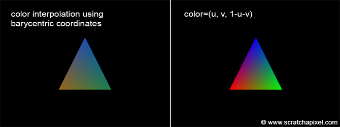
The complete implementation of this function is available in the source code section at the end of this lesson. As in the previous chapter, the program renders a single triangle and uses the barycentric coordinates of the intersection point to interpolate three colors across the triangle's surface.
Important Note on the Möller-Trumbore Algorithm Implementation: If you compile and run the code provided with this lesson, you might notice that the resulting image, when using the Möller-Trumbore algorithm, differs from the triangle image displayed above. This can be confusing because the image above was rendered using a geometric approach, not the Möller-Trumbore algorithm. The image below shows the outputs of the two algorithms side by side: the Möller-Trumbore solution is on the left, while the geometric solution is on the right.
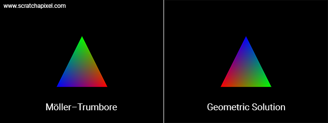
Mathematically, the two approaches are equivalent. The difference arises because the algorithms compute the barycentric coordinates \(u\), \(v\), and \(w\) in a different order (as explained earlier in this chapter). For example, the \(u\) coordinate in the geometric solution may correspond to \(w\) in the Möller-Trumbore solution, and so on. Thus, even though the resulting images may look different, both methods are correct. You may need to swap the coordinates when using them for texturing or shading.
Notes
One approach to accelerating the ray-triangle intersection is to store the constants \(A\), \(B\), \(C\), and \(D\) of the plane equation along with the triangle's vertices. These constants can be precomputed when the mesh is loaded and stored in memory for faster access. However, storing and accessing these variables in memory can sometimes be more costly than computing them on the fly, so this optimization does not always lead to a significant performance gain.
Another technique for speeding up the algorithm is to reduce the ray-triangle intersection problem to two dimensions. This is done by determining the dominant axis of the triangle's normal and using that information to select the two coordinates to use for the projection. This method is detailed in the paper *"Ray-Polygon Intersection: An Efficient Ray-Polygon Intersection"* (refer to the references section below).
There are also existing algorithms specifically designed for ray-tracing quadrilaterals (quads).
In our code, we use single-precision floating-point numbers, which are generally sufficient. However, the ray-triangle intersection test may encounter precision errors under certain conditions. For instance, the calculated intersection point may not lie exactly on the triangle's plane, and could be slightly above or below its surface. These precision issues will be discussed further in the lesson on shading.
As mentioned in the introduction to this lesson, there is another popular ray-triangle intersection routine that is widely used in modern production ray tracers, more so than the Möller-Trumbore algorithm. This method is presented in the paper *"Watertight Ray/Triangle Intersection"* by Ingo Wald, Sven Woop, and Carsten Benthin. This topic is covered in a separate lesson.
References
Fast, Minimum Storage Ray/Triangle Intersection. Möller & Trumbore. Journal of Graphics Tools, 1997.
Ray-Polygon Intersection. An Efficient Ray-Polygon Intersection. Didier Badouel from Graphics Gems I. 1990