Mathematical Foundations of Monte Carlo Methods

The Inverse Transform Sampling Method

This chapter is more of a general introduction to the inversion sampling method. Examples that are directly related to computer graphics will be presented in the next lessons (Monte Carlo Methods in Practice, Introduction to Sampling, and Introduction to Importance Sampling in particular).

The Inverse Transform Sampling Method

As explained in the previous paragraph, a CDF can be used to answer the question "what's the probability that a continuous random variable X takes on any value lower or equal to some number, where the number in question is somewhere within the boundaries of all the values that the random variable can take on. Is answering that sort of question useful in computer graphics? The answer is yes, but only indirectly.

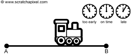
Let's use an example that we can understand without any prior knowledge of rendering and shading. Let's imagine that you wish to develop a train traffic simulator. You are interested in simulating one particular train which is going from point A to point B. While looking at real traffic data for this train, you have noticed that the time it takes to go from A to B can be anything between 25 to 35 minutes with an average of 30 minutes. If you divide the time between 25 and 35 into equal parts and count the number of trains that arrived in each one of these time slots (divided by the total number of trains), you might find that the curve you get looks very much like the normal standard distribution function we used earlier on in this chapter (this doesn't have to be, of course, we just used this function again because we are already familiar with it). In other words, the curve looks similar to that of figures 2 or 4 from the previous chapter (in red and black respectively), or the figure below. In this figure, we divided the time into slots of 1 minute but you would get a graph closer to the curve in black (the actual function/PDF) if you were to divide it into smaller bins.

What does this mean or to say it differently, how would you interpret this curve? Well, simply that it is more likely for instance for a train to arrive within 1 or 2 minutes of its scheduled arrival time than it is to arrive within 3, 4, or 5 minutes of that time. Understanding this is important. Expressed in terms of probability: the probability of the train arriving within 1 or 2 minutes of the scheduled time, is higher than the probability for that train to arrive within 3, 4, or 5 minutes of that time.

By the way, note that the time difference between the time the train has arrived and the average time can be considered as a continuous random variable contained within the lower and upper bound -5 (the train can't be more than 5' too soon) and 5 (the train can't be more than 5' too late), which we can write as:

Keep in mind that in probability this is called the sample space of the random variable. Now that we have this data in our hands, let's try to make a realistic train simulation. If you don't know much about probability and CDF, and just want to simulate the fact that the train generally doesn't arrive on time, you can add some small random offset to the train speed so that it arrives either too soon or too late (however on some occasion it might just arrive on time, that's just the nature of a random process). From a programming point of view, you can achieve this by simply drawing a random number between 25 and 35 and computing the train speed from that value (assuming you know the distance between A and B and that the train travels at a constant speed). Your virtual train will then arrive with potentially some time difference from the scheduled arrival time. Here is what the program looks like (the program is partially accurate because we should convert time in terms of minutes, seconds, etc. but for the sake of simplicity, we've ignored this detail):

#include <cstdlib> 
#include <cstdio> 
int main(int argc, char ** argv) 
{ 
    srand48(13);  //intialize uniform random variable 
    int numSims = 10; 
    const float dist = 10;  //10 km or miles 
    for (int i = 0; i < numSims; ++i) { 
        float time = 25 + drand48() * 10;  //any time between 25 and 35' 
        float speed = 60 * dist / time;  //km/miles per hour 
        printf("Train travel at speed: %f\n", speed); 
    } 
    return 0; 
} 

For those of you who are not familiar with C++, drand48() is a function that returns a random real number in the range 0 to 1\. Let's assume for now that we don't know how this function distributes these random numbers, or to say it differently, we don't know the probability with which drand48() generates these random numbers. This program though is a poor simulation of the real world. It might give you the illusion of randomness but does not simulate accurately real traffic data. Why? Each train that the simulation produces, arrives within a certain time of its scheduled arrival time. This is our random variable X. Let's call this time difference \(\Delta t\). Let's now divide the time interval [-5,5] into regular intervals or bins (100 intervals in the code below). For each train the simulation produces, we will remap \(\Delta t\) to its corresponding bin and increment its value (all bins are normalized at the end of the simulation, i.e. divided by the total number of trains). This will give us an indication of the way the random variable X (represented by \(\Delta t\)) is distributed by our program. Here is the new code:

#include <cstdlib> 
#include <cstdio> 
#include <cstring> 
 
int main(int argc, char ** argv) 
{ 
   srand48(13); 
   int numSims = 1000000; 
   int numBins = 100; 
   int bins[numBins]; 
   memset(bins, 0x0, sizeof(int) * numBins);  //set all the bins to 0 
   const float dist = 10;  //10 km 
   for (int i = 0; i < numSims; ++i) { 
       float diff = (2 * drand48() -1) * 5;  //random var between -5 and 5 
       int whichBin = (int)(numBins * (diff / 5 + 1) * 0.5); 
       bins[whichBin]++; 
       float time = 30 + diff; 
       float speed = 60 * dist / time; 
   } 
   float sum = 0; 
   for (int i = 0; i < numBins; ++i) { 
       float r = bins[i] / (float)numSims; 
       printf("%f %f\n", 5 * (2 * (i /(float)(numBins)) -1), r); 
       sum += r; 
   } 
   fprintf(stderr, "sum %f\n", sum); 
   return 0; 
} 

We now have the number of trains (divided by the total amount of trains) arriving within a certain time difference with respect to the average time. In probability, this is our probability distribution function (and because these are probabilities, if you sum them all up, you should get 1, which you can verify by running the program above). In other words, the result gives us the probability that a train arrives 5, 4, 3, 2, 1 too soon, on time or 1, 2, 3, 4, or 5 minutes too late. When we did this exercise before with real traffic data (see figure above), we found out that this curve (or graph) had the shape of a standard normal distribution function. If our simulation does the right thing (that is, if it produces data similar to real-world data which is the ultimate goal of any simulation), it should normally have the same probability distribution. Let's plot the data and look at the graph (the result of line 23):

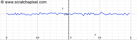
Disappointment! The curve is flat and not a bell-shaped curve. The probability distribution is uniform, and that's expected because in C/C++ the drand48() function is known to be a random generator with uniform distribution (the probability of getting any value between 0 and 1 is equal) and not a normal distribution as we need it to be.

From a programming point of view, let's say that we can only use this drand48() function which we know has a uniform probability distribution (however in C++11, the latest C++ standard, you can now find random number generators with various probability distribution functions, including a normal distribution but for the sake of this exercise we won't be using those). If you remember what we said about CDF, the function goes from 0 to 1 and is monotonically increasing. Since we can only generate a number between 0 and 1 with equal probability, what we could do, is draw a number using drand48() and look at it as being the result of the CDF. If you look at figure 1 which illustrates this idea, it must be clear that the probability of sampling any of the cubes making up the column is equal. Each cube has an equal probability to be chosen and any position on each one of these cubes has an equal probability to be chosen as well. Thus using a random variable with uniform distribution to pick a point anywhere along the Y-axis between 0 and 1 makes sense. If we say that \( r\) is the result of drand48() for example (in literature, random numbers with uniform distribution are often denoted with the Greek letter epsilon \(\epsilon \)), we could write:

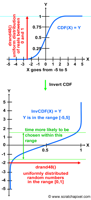
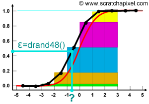
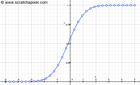
Let's see how this works with our example. In figure 2, we plotted the CDF of the standard normal distribution function (this PDF defines the probability that our train arrives within a certain time of the scheduled arrival time). As we know, the CDF converges to 1\. We can interpret the Y-axis of this graph, as the result of our random number generator with uniform distribution. Now, if we invert that graph (you can see the resulting graph at the bottom of figure 2), we get another graph in which the X-axis varies from 0 to 1 (previously Y in the top figure), and in which the Y-axis varies from -5 to 5 (previous X in the top figure). We inverted the CDF. If we then randomly chose a value for X between 0 and 1 (using drand48() for instance), what we get when we read the result of that function (in blue) for that value of X, is some random value (a value along the Y-axis) representing the time difference between the time the train shall arrive, and the time it is scheduled to arrive. Again, the Y value is random since the X value is random:

where \( y\) is a random number drawn from a "random number generator" with the PDF of interest. Which is what we wanted for our train simulation.

Spend some time looking at the graph, and try to see what happens for various values of X. You can see that the invert of the CDF for the normal distribution varies very little for small values of X (between 0 and 0.05) and value of X close to 1 (between 0.95 and 1). However since the values of X are chosen randomly and uniformly, it means that this function is more likely to return values between -2/-1.5 and 1.5/2 than between [-5,-2] or [2,5]. This is what we want, since we know by just looking at the PDF, that trains are more likely to arrive with a 1 or 2 minutes difference than with 3 or 4, or 5 (see in figure 4, the arrow with the annotation "time more likely to be chosen within that range").

So the next question is: how do we find the invert of the CDF? If your CDF is a function (such as the normal standard distribution function), in some cases, the inverse of that function may also exist in an analytical form. However, we don't want to be limited to cases where this inverse function exists, since we might as well in practical situations deal with arbitrary PDFs. Therefore, we need a generic solution. It happens that by discretizing the PDF, we can easily compute a "discretized" version of its associated CDF using for example the Riemann sum method and stacking up the samples as explained in the previous chapter. In code we get:

// standard normal distribution function
float pdf(const float &x) 
{ return 1 / sqrtf(2 * M_PI) * exp(-x * x * 0.5); } 
 
int main(int argc, char ** argv) 
{ 
    int nbins = 32; 
    float minBound = -5, maxBound = 5; 
    float cdf[nsamples + 1], dx = (maxBound - minBound) / nbins, sum = 0; 
    cdf[0] = 0.f; 
    for (int n = 1; n < nbins; ++n) { 
        float x = minBound + (maxBound - minBound) * (n / (float)(nbins)); 
        float pdf_x = pdf(x) * dx; 
        cdf[n] = cdf[n - 1] + pdf_x; 
        sum += pdf_x; 
    } 
    cdf[nbins] = 1; 
    printf("sum %f\n", sum); 
    for (int n = 0; n < nsamples + 1; ++n) { 
        printf("%f %f\n", minBound + (maxBound - minBound) * (n / (float)(nbins)), cdf[n]); 
    } 
    ... 
    return 0; 
}

When you create a CDF that way (in code) you need to be careful about the first and last samples which should be 0 and 1 as well as how you handle the other samples in between. Note that even though we discretized the PDF to construct the CDF, the CDF itself is still a continuous function. Let's graph what the program prints out (the values for the CDF from -5 to 5 which are the boundaries we chose for our PDF, the standard normal distribution function):

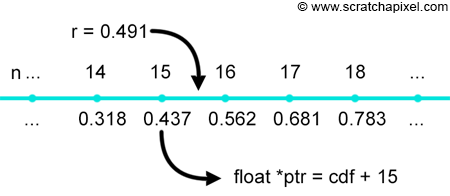
The next step is to produce a random number r with uniform distribution which we can do using some function like drand48() for example. We then use a C/C++ function called lower_bound which returns the first element in an array of numbers (in this case the floats making up the CDF), which value is lower than a given value (r). How this function works is illustrated in the following figure (r = 0.491). We can use this function of course because the CDF is a monotonically increasing piecewise-linear function (in other words, each sample in the series, is greater or equal in value to the sample preceding it in the array).

The address of the return pointer can be subtracted from the address of the first element of the array, which gives us the offset between the first element in the array and the element which is lower to r. In code we get:

#include <algorithm> 
int main(int argc, char ** argv) 
{ 
    ... 
    srand48(13); 
    float r = drand48(); 
    float *ptr = std::lower_bound(cdf, cdf + nbins + 1, r); 
    int off = (int)(ptr - cdf - 1); 
    printf("r %f offset %d\n", r, off); 
    printf("%f %f\n", cdf[off], cdf[off + 1]);  //r is contained within this bound 
    ... 
    return 0; 
}

We now know which are the two values bounding r (their respective indices in the array as well as their values of course which can easily access using these indices). As you can see in the figure below, the line between these two samples and the line between the lower bound sample (n=15) and r, can be seen as the hypotenuse of two similar triangles. We know from the lesson on Geometry, that the ratios of the lengths of similar triangles' corresponding sides are equal. In other words, we can write:

We then remap r between 0 and 1 (we call this value t but which is equivalent to DE in the figure below), such that:

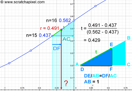
so that AB equals 1. DF is the distance we are looking at. It's the partial solution to our problem. We also know AC which is just the upper bound (5 in our example) minus the lower bound (-5 in our example) of the CDF divided by the total number of samples.

We can finally solve DF:

Finally, we can find x:

This is not the most elegant approach, but the most literal. It's better to think of the limits of the CDF to be in the range [0,1] and finally remap the resulting x to [min, max]. In other words:

As usual, the code version:

int main(int argc, char ** argv)
{
    ...
    float t = (r - cdf[off]) / (cdf[off + 1] - cdf[off]);
    printf("t %f\n", t);
    float x = (off + t) / (float)(nbins);
    x = minBound + (maxBound - minBound) * x;
    printf("x %f\n", x);
    ...
    return 0;
}

And for r (or y) = 0.491, we get x = -0.178. As you see without even explicitly inverting the CDF, we have a way of finding x for any given value of y. Let's now use this method for our train simulation. All we need to do is compute the CDF from the PDF (lines 28-35). Then, each time we need to simulate a new train, we call a function (line 11-19) in which we draw a random number in the range [0,1] with uniform distribution (line 13) and compute a random number with the desired PDF using the inverse sampling method we just described (line 14-18). As usual, to test the accuracy of our simulation, we will compute the number of trains arriving within certain slots of the scheduled arrival time. If the simulation does the right thing, we should get a bell-shaped curve, similar to that of the normal distribution function. Let's check.

#include <cstdlib> 
#include <cstdio> 
#include <cstring> 
#include <cmath> 
#include <algorithm> 
 
// standard normal distribution function
float pdf(const float &x) 
{ return 1 / sqrtf(2 * M_PI) * exp(-x * x * 0.5); } 
 
float sample(float *cdf, const uint32_t &nbins, const float &minBound, const float &maxBound) 
{ 
    float r = drand48(); 
    float *ptr = std::lower_bound(cdf, cdf + nbins + 1, r); 
    int off = std::max(0, (int)(ptr - cdf - 1)); 
    float t = (r - cdf[off]) / (cdf[off + 1] - cdf[off]); 
    float x = (off + t) / (float)(nbins); 
    return minBound + (maxBound - minBound) * x; 
} 
 
int main(int argc, char ** argv) 
{ 
     srand48(13);  //seed random generator 
     // create CDF
     int nbins = 32; 
     float minBound = -5, maxBound = 5; 
     float cdf[nbins + 1], dx = (maxBound - minBound) / nbins, sum = 0; 
     cdf[0] = 0.f; 
     for (int n = 1; n < nbins; ++n) { 
         float x = minBound + (maxBound - minBound) * (n / (float)(nbins)); 
         float pdf_x = pdf(x) * dx; 
         cdf[n] = cdf[n - 1] + pdf_x; 
         sum += pdf_x; 
     } 
     cdf[nbins] = 1; 
 
    // our simulation
    int numSims = 100000; 
    int numBins = 100;  //to collect data on our sim 
    int bins[numBins];  //to collect data on our sim 
    memset(bins, 0x0, sizeof(int) * numBins);  //set all the bins to 0 
    const float dist = 10;  //10 km 
    for (int i = 0; i < numSims; ++i) { 
	   float diff = sample(cdf, nbins, minBound, maxBound);  //random var between -5 and 5 
	   int whichBin = (int)(numBins * (diff - minBound) / (maxBound - minBound)); 
	   bins[whichBin]++; 
	   float time = 30 + diff; 
        float speed = 60 * dist / time; 
    } 
    sum = 0; 
    for (int i = 0; i < numBins; ++i) { 
        float r = bins[i] / (float)numSims; 
        printf("%f %f\n", 5 * (2 * (i /(float)(numBins)) -1), r); 
        sum += r; 
    } 
    fprintf(stderr, "sum %f\n", sum); 
    return 0; 
}

If we plot the data (line 53) we get the following graph:

This is exactly what we are expecting to see. The resulting curve looks like a normal distribution function.

Summary

Because this method is so important for anyone interested in shading and rendering, let's summarize what you should remember from this chapter. First, let's rephrase one more time the problem we are trying to solve. Our goal is to simulate a random process with a given probability density function or PDF. This PDF can be arbitrary especially if we try to simulate a real-world phenomenon for which we have acquired data. Understanding the concept of arbitrary PDFs is important. Some functions such as the normal distribution can be used as PDF. A list of common probability distributions can be found on Wikipedia. However not every real-world phenomenon random behavior can fit into one of these functions, in which case we say the PDF is arbitrary. Whether arbitrary or not, the properties of the PDF are always the same. The sum of the pdf for all values in the sample space is equal to 1 and it represents the relative likelihood for this random variable to take on a given value (as explained in the previous chapter).

Our need is to be able to draw a random variable with the same probability function. In other words, if real trains are more likely to arrive 1 minute before or after the scheduled arrival time than 2, 3, 4, or 5 minutes (the PDF), then when we draw random numbers to simulate the actual arrival time of a train, more of these numbers need to be closer to 1, than they will be to 2, 3, 4 or 5. This is what it means when we speak of drawing a random number with a given PDF.

The inversion method is a technique that can be used to achieve this goal. It works for an arbitrary PDF, in other words, the PDF doesn't have to be a known analytical function (such as the normal distribution function) to work. As long as we have data for that PDF, we can use this method. It consists of drawing a random number with uniform distribution. Let's call this random number \(\epsilon\). If we assume that this number is the result of the CDF, thus if we somehow can invert the CDF, we can write:

where \( x\) is a random number drawn from the desired probability distribution (the likelihood of a train arriving with some time difference from the scheduled arrival time). In this chapter, we showed that inverting the function is not necessary. In the code, we can find the result directly from the CDF.

The inversion method is fundamental in computer graphics, particularly for rendering, ray tracing, sampling, importance sampling, and Monte Carlo methods.

CDFs of Well-Known PDFs

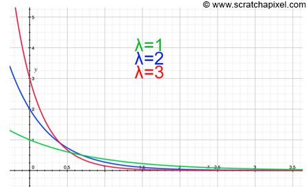
Interestingly enough, the CDF of some very useful functions in computer graphics can be found analytically. The only function we will look at in the version of this lesson is the exponential distribution (we will use it in the next lesson). As you can guess, the exponential distribution is a PDF based on the exponential function. It has the following form:

The variable \(\lambda\) (the Greek letter lambda) is called the rate of distribution. You can see a few plots of this function below for different values of \(\lambda\). Note that this PDF is only valid for values of x greater than 0.

This PDF is very common. For example, the decay of radioactive substances is exponential. If we want to compute the probability that a random variable X with exponential distribution is greater than some value t, we can find this probability by integrating the PDF from t to infinity:

If you don't remember how we can integrate function using the second law of calculus, check the chapter The Mathematics of Shading. Remember that the antiderivative of the exponential function is the exponential function itself (a quite extraordinary function indeed) and \( e^{-\infty} = 0\). Now, in most cases (at least in CG), we will be more interested in the probability of the random variable X being lower than t. We can write:

And this, in essence, is our CDF for the exponential distribution. Inverting this function is simple:

Remember that the inverse of the exponential function \( e^x\) is the natural logarithm \(\ln(x)\). The variable y in this equation is our uniformly distributed random variable \(\epsilon\), and since the variable is uniformly distributed, \(1 - \epsilon\) is similar to \(\epsilon\) from a probability point of view. Thus our inverted CDF reduces to:

This is a very important result. Any random variable with exponential distribution can be sampled using this function. All you need to do is draw a random number with uniform distribution, take the natural logarithm of that number and divide the result by the rate of distribution \(\lambda\) (which should be known).