Probability Distribution: Part 1
Reading time: 11 mins.Probability Distribution
The concept of probability distribution is very important (and play a central role in the importance sampling method). We introduce it here in this chapter rather than later, because, you should give to this concept and the concept of random variable the same attention, and actually see them both as part of a whole (or at least as being interconnected). Remember how we mentioned in the previous chapter that a random variable is some sort of function mapping outcomes to real values but also how probabilities are associated to these outcomes. For a die or a coin, the outcomes are equally likely to happen (where the outcomes can either be any number between 1 and 6, or heads or tails) thus we have shown in this case that the probability associated with each outcome is \(1\over n\), where \(n\) is the total number of possible outcomes (6 in the case of a die, 2 in the case of coin). Since each outcome has an associated probability (which you can see as a set of pairs of outcomes and their associated probabilities), we can plot these probability values vs. the possible outcome values. In statistics, this is what we call a probability distribution. We will give a more formal definition later on, but let's study a couple of cases first.
Example 1
When we used the example of a coin or a die in the previous chapter, we already introduced you somehow to the concept of probability distribution by showing you two graphs which we are reproducing here:
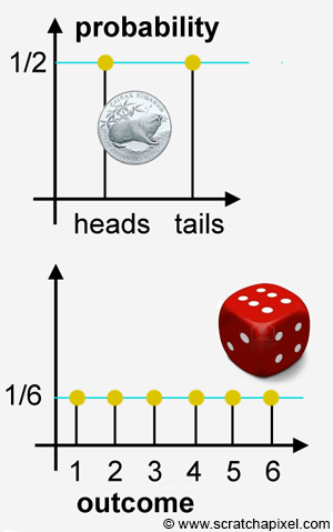
These probability distributions are pretty boring because each possible outcome from the experiment has the same probability. Probability distributions look more interesting though when the outcomes of an experiment have different probabilities. Let's study an example of such distribution. Remember the experiment we described in the previous chapter in which we had 10 cards, of which 3 were labeled with the number 0, 5 were labeled with the number 1, and 2 were labeled with the number 2. If you place these cards in a box, shake the box, etc. you will (hopefully) agree that each card in the box is equally likely to be randomly picked up. If we consider the sample as being \(S = \{0, 0, 0, 1, 1, 1, 1, 1, 2, 2\}\) (the order in this set doesn't matter, the numbers could be presented in a completely different order), then each outcome in this set has the associated probability \(1\over 10\). In probability theory, when we consider the probability of getting either one outcome or another, the probability of getting any of these two outcomes is the sum of their probabilities (we will study the properties of probability in the next chapter). This is known as the addition rule. In other words, if you were interested in knowing what is the probability of either getting a 2 or a 5 when you roll a die, this probability is the sum of getting a 2 (which we know is \(1\over 6\)) and the probability of getting a 5 (\(1\over 6\) again), that is \(2 \over 6\). Applied to our cards example, the probability of getting a card labeled 0 is the sum of the probabilities of each card in the set labeled 0, and the probability of getting a 1, is the sum of the probabilities of each card in the set labeled 1, etc. If we reduce our sample space to the space of elementary events then we get \(S = \{0, 1, 2\}\), and the probability of either getting a 0 a 1, or a 2 is \(3 \over 10\), \(5 \over 10\) and \(2\over 10\) respectively. If we now plot these probabilities as a function of the outcome, we get the following more interesting graph:
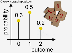
Note that the contrary of other functions, the dots corresponding to each pair outcome-probability are not linked because we are dealing in these particular cases with discrete random variables. For continuous random variables, the probability distribution function is represented as a curve (but more on this topic in the next lesson). Hopefully, with this example, you start to get the meaning of this function. It defines or describes a distribution of probabilities across the sample space of an experiment. When applied to discrete random variables, this function is called a probability mass function (or pmf). Here is finally a more formal definition of a probability distribution.
In probability and statistics, a probability distribution assigns a probability to each measurable subset of the possible outcomes of a random experiment. The distribution can be discrete, or continuous. A discrete distribution can be characterized by its probability (distribution) function, which specifies the probability that the random variable takes each of the different possible values.
Before we move to the next example, note how the sum of all the probabilities is equal to 1\. Indeed we will show in the next chapter that this is a property of probabilities. A probability can never be greater than 1 and the probabilities of an experiment sum to 1.
Example 2
In probability theory when a random process has only two outcomes (such as "heads" or "tails", "success" or "failure") then we speak of a Bernoulli (or binomial) trial. In the coin experiment, these two outcomes occur with the same probability (\(\scriptsize p = {1 \over 2 }\)) but in the more generic case, we say they occur with probability p and 1 - p (the sum of probabilities is 1). But what is for example the probability of getting 4 heads if I toss the coin 6 times? Note that the possible outcomes of this experiment (tossing 6 times and counting heads) can now either be 0, 1, 2, 3, 4, 5, or 6\. First, if you now consider an experiment in which \(n\) random samples are drawn from, the probability distribution of a Bernoulli trial, where each sample can take a value of 0 or 1, then the sum of this \ (N\) samples can be written as:
$$S = \sum_{i=1}^N x_i$$Let's say that we want to find the probability that \(S = n\), where \(n \leq N\), which is the probability that \(n\) of the \(N\) samples take on the value of 1, and \(N- n \) samples take on the value of 0\. In mathematics, this discrete (because \(n\) takes on discrete values) probability distribution is called a binomial distribution and can be analytically calculated with the following equation:
$$Pr(S = n) = C_n^N p^k(1-p)^{(N-n)}$$for n = 0, 1, 2, ..., N, where:
$$C_n^N = {{N!}\over{n!(N-n)!}}.$$The expression \(x!\) is called the factorial of x. It is equal to the product of all positive integers less than or equal to x. For example: \(\scriptsize 5! = 5 * 4 * 3 * 2 * 1 = 120\). The term \(C_n^N\) counts the number of ways in which \(n\) of the \(N\) samples can take on the value of 1. In the case of a fair coin probability p is equal to \(1\over 2\). In our example, we toss the coin 6 times thus n=6, and k can take any value between 0 and 6\. For example, if we set k=3, the binomial distribution would give us the probability that we would get 3 heads if we were to flip the coin 6 times. We can write a small C++ program to compute all the probabilities for each value of k between 0 and 6:
#include <random>
#include <cstdlib>
#include <cstdio>
#include <iostream>

inline uint64_t fact(uint64_t x) {
  return (x <= 1 ? 1 : x * fact(x - 1));
}

int main(int argc, char **argv)
{
    uint64_t N = atoi(argv[1]);
    uint64_t Nfac = fact(N);
    for (uint64_t n = 0; n <= N; ++n) {
        uint64_t CnN = Nfac / (fact(n) * fact(N-n));
        double prob = CnN * powf(0.5, n) * powf(1 - 0.5, N - n);
        std::cout << n << " " << prob << std::endl;
    }

    return 0;
}

We show the result as a graph in Figure 1. The resulting numbers can be seen as the frequency of getting a certain random variable. For example, the first column gives us the frequency of getting no heads after 6 tosses (this probability is 0.015625). The second column gives the probability of getting 1 head after 6 tosses (0.093750), etc. Another way of seeing this is to say that 1.5% of the time you will get 0 heads, 9.3% of the time you will get 1 head, 23% of the time you will 2 heads, 31% of the time you will get 3 heads, etc.
The reason we studied this example is to show that in example 1 we could easily compute the probability distribution of our random distribution by hand (because the experiment was simple enough), but for some more complex or typical cases, this probability distribution can be computed using mathematical equations (where the parameters of these equations are the experiment's parameters such as how many times do we toss the coin, what's the probability to get "success" in a Bernoulli trial, etc.). And as in any other mathematical equation, changing these parameters do change the "shape" of the probability distribution. Look at this series of three graphs, made from using the binomial distribution equation with different values for the parameter \(N\):
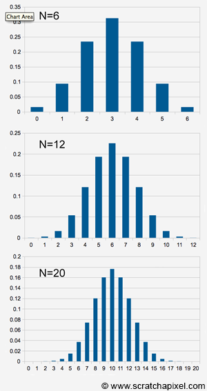
The values for the probabilities here are not so important. It doesn't matter if you can't read the numbers, all we want you to understand is that the overall shape of the distribution changes as the parameters of the equation change. There is more we could say by just looking at these distributions themselves (for example that they are symmetrical about their central value, either 3, 6, or 10 when the N is set to 6, 12, and 20 respectively, etc.) but let's ignore these observations for now and keep the focus on the idea that some probability distributions can be defined with mathematical equations and that by varying the values of these equations' parameters we can change their shapes. We gave the example of the binomial distribution, but how many more types of distribution can we define using equations? There are quite a few but what's probably the most interesting remark to make about this is that some probability distributions in nature are very common and probability one of the most common and useful ones is known as the normal or gaussian distribution. The normal distribution is very similar to the binomial distribution but where the binomial distribution applies to discrete random variables, the normal distribution applies to continuous random variables. We won't provide the equation for the normal distribution in this chapter because it uses two parameters called the mean and the standard deviation which we haven't introduced yet (check the chapter probability distribution: part 2 to get the equation). But these concepts will be explained in the next chapter. For now, we will just show what the normal distribution looks like:
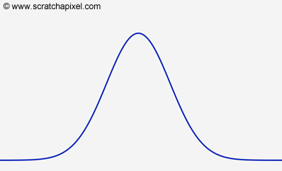
It doesn't matter at this point if you don't know how to create this curve, just compare its shape with the shape of the three binomial probability distributions shown above, especially with the graph at the bottom (when N=20). You can see that the overall shape is the same. As mentioned, the normal probability distribution is the counterpart of the binomial distribution for continuous random variables (thus logically they do have the same shape, but rather than just being discrete pairs, probabilities are expressed as a curve).
The other basic probability distribution which we have already been exposed to with the example of the die and the coin is called the discrete uniform distribution (its continuous counterpart is given the name of continuous uniform distribution). This distribution applies to any experiment in which each of the possible outcomes is equally likely to happen, and every one of these \(n\) outcomes has probability \(1\over n\). A simple sample space is given to a sample space in which the probability assigned to each outcome \(s_1, s_2, ..., s_n\) is \(1\over n\). Another common probability distribution in computer graphics is the Poisson distribution but don't worry too much about it for now. We will come across this name again when we get to the lesson on sampling. A list of probability distributions can be found here.
Before we can study some of the properties of a probability distribution that are useful to understand the Monte Carlo method, we first need to learn more about the properties of probabilities, as well as introduce some important concepts from probability theory and statistics. Let's move on to the next chapter then.