Mathematical Foundations of Monte Carlo Methods

Probability Density Function (PDF) and Cumulative Distribution Function (CDF)

The concepts of PDF (probability density function) and CDF (cumulative distribution function) are very important in computer graphics. Because they are so important, they shouldn't be buried into a very long lesson on Monte Carlo methods, but we will use them in the next coming chapters, and thus, they need to be introduced at this point in the lesson. If you are serious about rendering and shading (from a programming point of view), this is a chapter we recommend you read carefully. We are likely to refer to this page quite often and even re-introduce those concepts in other lessons, to give them more visibility.

The Probability Distribution Function or PDF

In the previous chapters, we already introduced the concept of probability distribution. In short, a probability distribution assigns a probability to each possible outcome of a random experiment. We also suggested that a random variable could either be discrete or continuous. The number you get from throwing a die is an example of a discrete random variable and the amount of rain falling in London is an example of a continuous random variable (the amount of water falling at any given time can be measured of course, but this number can be anywhere within a given range while in the case of a dice, it can only take on a fixed value, either 1, 2, 3, 4, 5 or 6).

In chapter 3 (in which we introduced the concept of the probability distribution), we mentioned that the function known as the binomial distribution, could be used to compute the probability of the number of successes in a sequence of n independent yes/no experiments (for example "the probability of getting 3 heads, when a coin is tossed 6 times"). When a function defines a discrete probability distribution (such as in the example we just provided), we call this function a probability mass function (or pmf). Let's now look at the continuous case. The height of adults in a particular ethnic group is a continuous random variable which in general, follows more or less, a normal distribution. It is a continuous variable because height is not something that is discretized as in the case of the numbers of a dice. The concept of normal or gaussian distribution was introduced in chapter 8. It is a function defined by two parameters, a mean and a standard deviation. When a function such as the normal distribution defines a continuous probability distribution (such as the way height is distributed among an adult population), this function is called a probability density function (or pdf). In other words, pdfs are used for continuous random variables and pmfs are used for discrete random variables. In computer graphics, we almost always deal with pdfs. In short:

• The probability mass function (pmf) is the probability distribution of discrete random variable.

• The probability distribution function (pdf) is the probability distribution of a continuous random variable.

In mathematical notation, X ~ D means the random variable X has the probability distribution D.

The Cumulative Distribution Function or CDF

The notion of Cumulative Distribution Function or CDF is probably one of the most important and useful concepts from the entire field of probability theory when it comes to Monte Carlo methods applied to computer graphics. Why? The rendering of CG images involves many integrals which are very hard to efficiently evaluate by any other means than a method called the Inverse Sampling Method and this method is based on CDF (we will study the Inverse Sampling Method later in this chapter). Both the concept of PDF and CDF are central to the field of rendering in computer graphics. We recommend you study them well, which shouldn't be hard, because they are pretty simple (and yet powerful) tools.

In the example below (Figure 2), we have drawn the curve of the standard normal distribution function. The function is just a particular case of the normal (or gaussian) distribution function for which the parameters \(\mu\) and \(\theta\) (its mean and standard deviation) are respectively equal to 0 and 1\. We introduced this function in a previous chapter of this lesson). The choice of a function here is not important. Any other probability density function could be used. Remember though that one of the main and most important properties of PDFs (as well as PMFs) is that the sum of probabilities must equal 1. If g(x) is such a function (in other words a PDF), then:

In this case, g(x) represents the PDF of a continuous random variable as explained at the beginning of this chapter, however, keep in mind that this is also true when the random variable is discrete (if you sum up the probability of each possible outcome, you get 1). Incidentally, one of the properties of the normal distribution, is that its integral is 1 (which is good since we need this to use this function as a PDF).

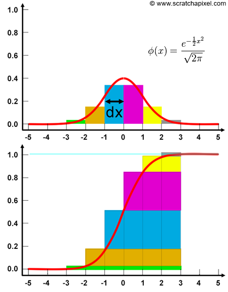
In the lesson on Shading [link], we learned about integrals and we also learned how to numerically evaluate integrals using the Riemann sum technique. The idea consists of evaluating the function at regular intervals within the boundaries of the integral's domain of integration, multiplying each one of these numbers by the distance between two intervals, and summing them up. The smaller the distance between two consecutive intervals, the more accurate the approximation. We also illustrated this idea in Figure 2 (where dx=1in this example)

Even though the domain of integration goes from minus to plus infinity, because the function is very close to zero outside the range [-5,5], it is acceptable to just consider values within that range. To keep the demonstration simple, we will also just evaluate the normal distribution function at 10 regular intervals within that range. In practice, you would probably want more samples to get a more accurate approximation. Here is a result of our PDF for these 10 samples (first row: sample index, second row: x values, third row: the result of the standard normal distribution function g(x)):

Now in this table, we rounded the numbers of the third row to the third decimal place, but if you run the program below, you can get the exact values. If you multiply each one of these numbers by the distance between each sample (dx=1 in this case) and sum them up, you get 1, as expected (not all PDFs might give you exactly 1. The standard normal distribution function has the particularity to always sum up to 1 regardless of the number of samples taken. When only a few samples are taken, integrating PDFs using the Riemann sum method only gives values close to 1 but as mentioned before, as you increase that number of samples, the sum should keep getting closer to 1. In other words, the sum of the samples will converge to 1 for all PDFs as the number of samples gets to infinity). You can check this result by compiling and executing the following program:

#include <cstdio> 
#include <cstdlib> 
#include <cmath> 
int main(int argc, char **argv) 
{ 
    int numIter = 10; 
    float minBound = -5, maxBound = 5; 
    float cdf = 0, dx = (maxBound - minBound) / (float) numIter; 
    for (int i = 0; i < numIter; ++i) { 
        float x = minBound + (maxBound - minBound) * (i + 0.5) / (float)numIter; 
        float g_x = 1 / sqrtf(2 * M_PI) * exp(-(x * x) / 2); 
        printf("%f %f\n", x, g_x); 
        cdf += g_x * dx;  //add current sample to all previous samples 
        printf("CDF at %f: %f\n", x, cdf); 
    } 
    printf("Sum: %f\n", cdf);  //the final sum should be 1 
    return 0; 
} 

Computing the CDF itself is as simple as adding the contribution of the current sample to the sum of all previous samples that were already computed (line 13 of our program). Keep in mind that we use this technique to compute the CDF of a PDF which is by definition a continuous function. Thus even though our method results in a series of discrete samples, the CDF is itself a continuous function. With only a few samples, we get a pretty crude representation of what that CDF should be (as in Figure 2 where you can see how the rectangles give a very approximate shape of the CDF for the standard normal distribution function), however, of course, the more samples you use, the closer you get to its actual "true" shape. This is illustrated in the following figure in which you can see the CDF of the function approximated with 10 samples (red) and 30 samples (green) compared to the actual CDF (in blue). As you can see the more samples, the closer we get to the actual CDF.

So the real question now. What are CDFs useful for? In probability theory they are useful for computing things such as "what is the probability of getting any of the first N possible outcomes of a random variable X". Let's take an example. We know that a dice has 6 possible outcomes, it could either be 1, 2, 3, 4, 5, or 6. And we also know that each of these outcomes has a probability 1/6. Now, if we want to know the probability of getting any number lower or equal to 4 when we throw these dice, what we need to do, is sum up the probability of having a 1, a 2, a 3, and a 4. We can write this mathematically as:

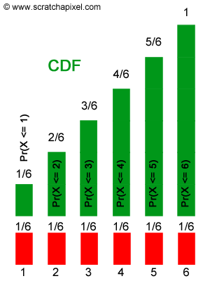
We have summed up the probabilities of the first N given possible outcomes (where N in this example is equal to 4). If we plot the result of this summation for Pr(X <=1), Pr(X <= 2), ... up to Pr(X <= 6), we get the diagram in Figure 4, which as you can guess, is the CDF (in green) of the probability function (in red) of our random variable. It is easier to explain the use of CDFs using a discrete random variable (our dice example), however, keep in mind that the idea applies to both discrete and continuous probability functions. For example, If we say that the standard normal distribution is the PDF of any given continuous random variable X, then we now know how to use its CDF to answer a question such as: what is the probability that X takes on any value lower or equal to 0?

The answer is the sum of all the probabilities for this random variable X to take on any value lower or equal to 0. We also know that the PDF is the function that "describes" the probability of these "continuous" outcomes. Thus all we need to do is, sum up this probability from say -5 to 0 (as explained before we chose -5 because the PDF is very close to 0 for any value lower than -5). To do that, we can use the Riemann sum method for example, which we described earlier. If you look at the blue curve in Figure 3 (which is the actual CDF of the standard normal distribution function), then you can see that at x = 0, the CDF is equal to 0.5. Thus, the answer to this question is 0.5.

This is an example of what CDFs are useful for, but they are most useful to us (as in people interested in computer-generated graphics) for their use in a technique called the inverse transform sampling method we are now going to describe.