Probability Properties
Reading time: 9 mins.Mutually Exclusive and Collectively Exhaustive Events
Generally, when you study probability theory, you spend quite some time studying things related to sets (more generally set theory). A sample space, as explained in the first chapter is an example of a set. There is a whole list of theorems and properties which are related to sets such as what is a union or an intersection of two sets, etc. but we won't be learning about them here (because they are not so important for us and pretty boring we have to admit). The concept of mutually exclusive events though is an exception and you need to know about it. Two sets A and B are said to be mutually exclusive or disjoint (the two terms mean the same thing) if A and B have no elements in common. For example \(A = \{1, 2, 3\}\) and \(B = \{4, 5, 6\}\) are two mutual exclusive or disjoint sets. When applied to the concept of the event, we say that two events are mutually exclusive (or disjoint) if they cannot both occur at the same time. Be careful not to confuse this concept with the concept of independent events (see below).
Another important concept however slightly easier to explain, is the concept of collectively exhaustive events. A set of events (such as the number of a die) is said to be jointly or collectively exhaustive if at least one of the events must occur.
This becomes a bit more complex when you start to combine concepts of mutually exclusive and collectively exhaustive events together (a mouthful of mathematical expressions). For example, we know that 1, 2, 3, 4, 5, and 6 are the possible outcomes of a die roll. Thus, in this case, we can say that the events from that set are collectively exhaustive because when we roll a die we are sure to get either one of these numbers (and nothing else than these numbers). However, if you consider a set made of outcomes 1 and 6, the events are mutually exclusive (because they can't occur at the same time) but they are not collectively exhaustive (because you might get a different number such as 2, 3, 4 or 5, thus you don't have the guarantee that you will get either 1 or 6). Tossing a coin is an example of experiment-producing events that are both mutually exclusive and collectively exhaustive; of the two possible outcomes (you need at least two outcomes to define a random process, if you only have one then it's deterministic) you are sure to either get one or the other (thus they are collectively exhaustive) and if you get "heads" you can't get "tails" (thus they are mutually exclusive).
Properties of Probabilities
If you remember the definition we gave to probability in the first chapter, the probability Pr(A) for the event A to occur, where A is one of the possible outcomes from the sample space of an experiment, then to be valid, Pr(A) (the probability that A will occur) needs to satisfy three axioms:
-
Axiom 1: first for every event A, \(Pr(A) \ge 0\),
-
Axiom 2: if an event is certain to occur, then the probability of that event is 1.
-
Axiom 3: the third axiom relates to the additive property of probability which we have already talked about in chapter 1\. It states that If two events are mutually exclusive (we explained what mutually exclusive events are above), then the probability that one or the other will occur is the sum of their probabilities. To be formal, you can say that any countable sequence of mutually exclusive \(E_1, E_2, ...\) events satisfy: $$Pr(E_1 \cup E_2 \cup \;...) = \sum_{i=1}^\infty Pr(E_i).$$ In set theory, the \(\cup\) symbol which is used to denote unions can be read as "or". For example, the union of two sets A and B (which you write \(A \cup B\)) is the collection of points that are in A or in B or in both A and B. We have already given an example of an application of this axiom in the first chapter.
For the rest of this chapter we will consider that all the experiments we are dealing with a finite sample space, in other words, we will only consider experiments that have a finite number of possible outcomes (their sample space S contains a finite number of elements \(s_1, s_2, ..., s_n\)). If you now consider that probability \(p_i\) is associated with the outcome \(s_i\) from the sample space S (where \(i = 1, 2, ..., n\)), then the probabilities \(p_1, p_2, ..., p_n\) must satisfies the following conditions:
\(p_i \ge 0\) for \(i = 1, ..., n\)
and
\(\sum_{i=1}^n p_i = 1\).
Remember from lesson 15 (Mathematics of Shading) that the \(\sum\) symbol is synonymous with sum. In other words, the sum of all probabilities associated with each possible event of an experiment is always one (the sum of each probability associated with each number of a six-sided die, 6 times 1/6, is 1).
From these axioms, you can deduce a few more useful properties. If you consider an experiment in which each outcome is equally likely to happen (where the probability of each outcome is \(1 \over n\) and \(n\) is the number of possible outcomes), then if an event A in the sample space of this experiment contains exactly \(m\) outcomes, then \(Pr(A) = {m \over n}\) (in other words, in a simple sample space S, the probability of an event A is the ratio of the number of outcomes in A to the total number of outcomes in S). If you consider the probability of getting an odd number in a die roll, where here m=3 and n=6, then Pr(odd)=3/6\. A couple more consequences: if a set of events A is a subset of a set of events B (which in mathematics we denote \(A \subseteq B\)) then \(Pr(A) \le P(B)\). This is known as the monotonicity property. And finally, the probability that an event E will occur can only be greater or equal to zero and lower or equal to one: \(0 \le Pr(E) \le 1\). This is known as the numeric bound property. If an event never occurs, its probability is 0 and if it always occurs, its probability is 1.
There is one last theorem that is important for us, people interested in 3D rendering. It is known as the multiplication rule. It is not necessary to know about it to understand the Monte Carlo method, but since this is the lesson in which we talk about probability in general and since we will be using this theorem later in the course of these tutorials (when we will learn about a technique called Russian roulette), we will introduce it here. To understand the multiplication rule you need to consider an experiment in which for example we toss a coin two times. Imagine you note whether you got "heads" or "tails" on the first and the second toss. The question is now, "what's the probability to get HH?" (where H denotes heads and T "tails"), in other words, what is the probability that we can get two heads in a row? The following figure (called a probability tree) might help you get an intuition about what the answer is to this question:
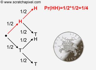
The chances of getting "heads" after the first toss are \(1 \over 2\). Because the events are mutually exclusive, your chances to get "heads" on the second toss are still 50 percent, however, the combined probability of getting heads twice in a row is the probability of getting "heads" the first time multiplied by the probability of getting heads the second time that is \(1 \over 4\). This is maybe easier to understand if you look at the probability tree above. The probability of getting "heads" or "tails" for each toss is the same, however, the probability of getting a particular sequence of "heads" and "tails" is the result of the probability of each outcome in the sequence multiplied by each other. In other words, if we want to find out the probability of getting the sequence HHT for instance we would have to multiply the probability of getting H multiplied by the probability of getting H again multiplied by the probability of getting T, that is \( {1 \over 2 } * {1\over 2} * {1 \over 2} = {1 \over 8} \). This is only true though when the events in the sequence are independent of each other (see below). Readers interested in this theorem can search for conditional probabilities.
Independent Events
When you toss a coin the probability of getting heads or tails is \(1\over 2\) as we know it, but if you toss the coin a second time, the probability of getting either heads or tails is still \(1\over 2\). In other words, the first toss did not change the outcome of the second toss or to say it differently again, the chances of getting heads or tails on the second toss are completely independent of whether or not we got "tails" or "heads" in the first toss. And this, of course, has nothing to do with the number of times you toss a coin. If you got 5 heads in a row (even though unlikely but still possible at least from a probability point of view), on the sixth time, your chances of getting "heads" or "tails" are still 50-50 and this is what you call disjoint or mutually exclusive events. Events are independent of each other or and that might be a more formal definition of what independent events are, if knowing that some event B has occurred does not change the probability of A, then A and B are said to be independent. When events are independent then it follows from the multiplication rule we have introduced above that \(Pr(A \cap B) = Pr(A)Pr(B)\). The symbol \(\scriptsize \cap\) in set theory means intersection. You can read the expression as the probability of getting A and B is equal to the product of the individual probabilities for A and B.